基于LSTM的温度时序预测

1.背景

本文接【时序预测SARIMAX模型】 一文，采用LSTM模型进行平均温度数据预测。具体的背景和数据分析就不做重复说明，感兴趣可以去看上文即可。

2.LSTM模型

RNN（Recurrent Neural Network，循环神经网络）是一种特殊的神经网络，被广泛应用于序列数据的建模和预测，如自然语言处理、语音识别、时间序列预测等领域。RNN对时间序列的数据有着强大的提取能力，也被称作记忆能力。相对于传统的前馈神经网络，RNN具有循环连接，可以将前一时刻的输出作为当前时刻的输入，从而使得网络可以处理任意长度的序列数据，捕捉序列数据中的长期依赖关系。

图 1

LSTM（Long Short-Term Memory，长短时记忆网络）是一种特殊的 RNN，它通过引入门控机制和记忆单元等结构来增强 RNN 的记忆能力和表达能力。

LSTM 的基本结构包括一个循环单元和三个门控单元：输入门、遗忘门和输出门。循环单元接受当前时刻的输入和前一时刻的输出作为输入，并输出当前时刻的输出和传递到下一时刻的状态。输入门控制当前时刻的输入对状态的影响，遗忘门控制前一时刻的状态对当前状态的影响，输出门控制当前状态对输出的影响。记忆单元则用于存储和传递长期的信息。基于此，使得LSTM具有长期的记忆能力，并且具有防止梯度消失的特点，故我们选择LSTM作为库存预估模型的训练基础。

图 2

3.模型训练

3.1 查看数据信息

df.info()

<class ‘pandas.core.frame.DataFrame’>
DatetimeIndex: 1462 entries, 2013-01-01 to 2017-01-01
Data columns (total 9 columns):
# Column Non-Null Count Dtype
->-- ------ -------------- -----
0 meantemp 1462 non-null float64
1 humidity 1462 non-null float64
2 wind_speed 1462 non-null float64
3 meanpressure 1462 non-null float64
4 year 1462 non-null int32
5 month 1462 non-null int32
6 day 1462 non-null int32
7 dayofweek 1462 non-null int32
8 date 1462 non-null object
dtypes: float64(4), int32(4), object(1)
memory usage: 91.4+ KB

3.2 数据分析

从【时序预测SARIMAX模型】 中可以看到温度数据具有明显的周期特征，因此需要考虑做归一化。

from sklearn.preprocessing import RobustScaler, MinMaxScaler

robust_scaler = RobustScaler()   # scaler for wind_speed
minmax_scaler = MinMaxScaler()  # scaler for humidity
target_transformer = MinMaxScaler() 

dl_train['wind_speed'] = robust_scaler.fit_transform(dl_train[['wind_speed']])  # robust for wind_speed
dl_train['humidity'] = minmax_scaler.fit_transform(dl_train[['humidity']]) # minmax for humidity
dl_train['meantemp'] = target_transformer.fit_transform(dl_train[['meantemp']]) # target

dl_test['wind_speed'] = robust_scaler.transform(dl_test[['wind_speed']])
dl_test['humidity'] = minmax_scaler.transform(dl_test[['humidity']])
dl_test['meantemp'] = target_transformer.transform(dl_test[['meantemp']])

display(df.head())
display(dl_train.head())

图 3

3.3 数据准备

from tensorflow.keras.models import Sequential
from tensorflow.keras.callbacks import EarlyStopping

def create_dataset(X, y, time_steps=1):  
    Xs, ys = [], []   
    for i in range(len(X) - time_steps):   
        v = X.iloc[i:(i + time_steps)].values 
        Xs.append(v)      
        ys.append(y.iloc[i + time_steps])
    return np.array(Xs), np.array(ys)  

sequence_length = 3  # adjust based on your dataset and experimentation
X_train, y_train = create_dataset(dl_train, dl_train['meantemp'], sequence_length)
X_test, y_test = create_dataset(dl_test, dl_test['meantemp'], sequence_length)

3.4 构建模型及评估

from tensorflow.keras.layers import LSTM,Dropout,Dense

# Build the LSTM model
lstm_model = Sequential()
lstm_model.add(LSTM(100, activation='tanh', input_shape=(sequence_length, X_train.shape[2])))
# lstm_model.add(LSTM(128, activation='softsign', input_shape=(sequence_length, X_train.shape[2])))
lstm_model.add(Dropout(0.5))
lstm_model.add(Dense(1))
lstm_model.compile(optimizer='adam', loss='mse')

# Define early stopping callback
early_stopping = EarlyStopping(monitor='val_loss', patience=10, restore_best_weights=True)

# Train the model
history = lstm_model.fit(X_train, y_train, epochs=30, validation_data=(X_test, y_test), batch_size=1, callbacks=[early_stopping])

# Evaluate the model
loss = lstm_model.evaluate(X_test, y_test)
print(f'Validation Loss: {loss}')
lstm_model.summary()

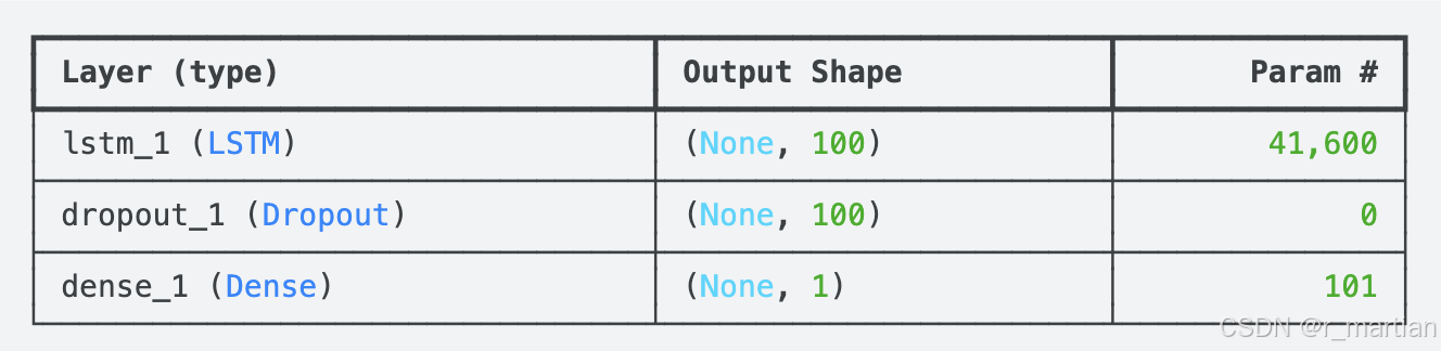
图 4

3.5 模型预测

# Make predictions
lstm_pred = lstm_model.predict(X_test)
lstm_pred = target_transformer.inverse_transform(lstm_pred)  # Inverse transform to original scale

# Inverse transform the true values for comparison
y_test = y_test.reshape(-1, 1)
y_test = target_transformer.inverse_transform(y_test)

3.6 模型评估

# Calculate RMSE and R2 scores
from sklearn.metrics import mean_squared_error, r2_score, mean_absolute_error

rmse = np.sqrt(mean_squared_error(y_test, lstm_pred))
r2 = r2_score(y_test, lstm_pred)

print(f'RMSE: {rmse}')
print(f'R2 Score: {r2}')

# Plot the results
plt.figure(figsize=(14, 7))
plt.plot(df.index[-len(y_test):], y_test, label='True Values')
plt.plot(df.index[-len(y_test):], lstm_pred, label='Predictions', linestyle='dashed')
plt.xlabel('Date')
plt.ylabel('Mean Temperature')
plt.title('Mean Temperature Predictions vs True Values')
plt.legend()
plt.show()

# Get training and validation losses from history
training_loss = history.history['loss']
validation_loss = history.history['val_loss']

# Plot loss values over epochs
plt.plot(training_loss, label='Training Loss')
plt.plot(validation_loss, label='Validation Loss')
plt.xlabel('Epoch')
plt.ylabel('Loss (MSE)')
plt.title('Training and Validation Loss')
plt.legend()
plt.show()

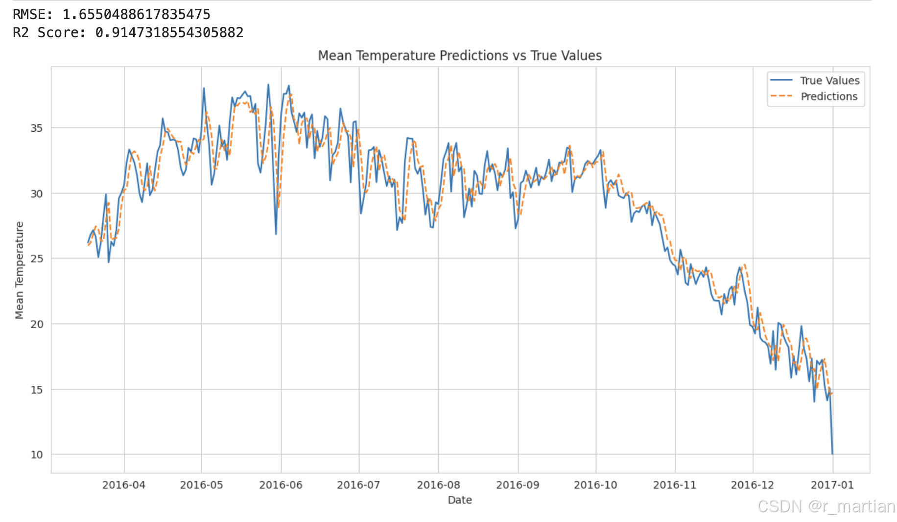
图 5

图 6

从结果看，模型拟合的效果还可以，相比于模型默认参数，做了一些参数调教，比如网络层数、激活函数以及Dropout等，还有一些参数尝试过调整，效果都一般，主要是对比不同参数下RMSE和R2两个值。后续出一些关于模型调参的文章，本文完。

参考文档

1. https://colah.github.io/posts/2015-08-Understanding-LSTMs/
2. https://www.kaggle.com/code/kevintinker1/time-series-forecasting-with-lstm
3. 携程基于LSTM的广告库存预估算法

如有侵权，烦请联系删除

原文地址：https://blog.csdn.net/cjqh_hao/article/details/142426920

免责声明：本站文章内容转载自网络资源，如本站内容侵犯了原著者的合法权益，可联系本站删除。更多内容请关注自学内容网（zxcms.com）！