趋势（一）利用python绘制折线图

🕗 发布于 2024-10-16 13:18 python 数据可视化

趋势（一）利用python绘制折线图

折线图（ Line Chart）简介

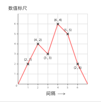
折线图用于在连续间隔或时间跨度上显示定量数值，最常用来显示趋势和关系（与其他折线组合起来）。折线图既能直观地显示数量随时间的变化趋势，也能展示两个变量的关系。

快速绘制

基于matplotlib

import matplotlib.pyplot as plt
import numpy as np

# 自定义数据
values = np.cumsum(np.random.randn(1000,1))

# 绘制折线图
plt.plot(values)
plt.show()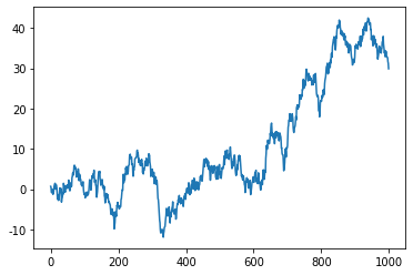

基于seaborn

import seaborn as sns
import matplotlib.pyplot as plt
import numpy as np

# 自定义数据
values = np.cumsum(np.random.randn(1000,1))

# 绘制折线图
sns.lineplot(x=np.array(range(1, 1001)), y=values.ravel())  # 使用 ravel() 将 values 转化为一维
plt.show()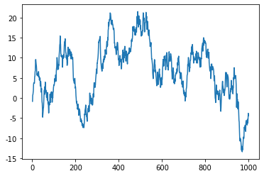

基于plotly

import plotly.graph_objects as go
import numpy as np

# 自定义数据
values = np.cumsum(np.random.randn(1000,1))

# 绘制折线图
fig = go.Figure(data=go.Scatter(x=list(range(1, 1001)), 
                                y=values.ravel(), 
                                mode='lines'))
fig.show()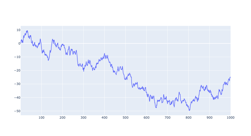

基于pandas

import numpy as np
import matplotlib.pyplot as plt
import pandas as pd

# 自定义数据
values = np.cumsum(np.random.randn(1000,1))
df = pd.DataFrame(values, columns=['Values'])

# 绘制折线图
df.plot()
plt.show()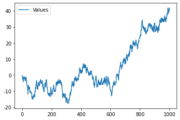

定制多样化的折线图

自定义折线图一般是结合使用场景对相关参数进行修改，并辅以其他的绘图知识。参数信息可以通过官网进行查看，其他的绘图知识则更多来源于实战经验，大家不妨将接下来的绘图作为一种学习经验，以便于日后总结。

通过matplotlib绘制多样化的折线图

matplotlib主要利用plot绘制折线图，可以通过matplotlib.pyplot.plot了解更多用法

修改参数

import matplotlib as mpl
import matplotlib.pyplot as plt
import numpy as np
import pandas as pd

plt.rcParams['font.sans-serif'] = ['SimHei'] # 用来正常显示中文标签

# 自定义数据
df=pd.DataFrame({'x_values': range(1,11), 'y_values': np.random.randn(10) })

# 初始化布局
fig = plt.figure(figsize=(12,3))

# 自定义颜色
plt.subplot(1, 3, 1) 
plt.plot( 'x_values', 'y_values', data=df, color='skyblue')
plt.title('自定义颜色')

# 自定义透明度
plt.subplot(1, 3, 2) 
plt.plot( 'x_values', 'y_values', data=df, color='skyblue', alpha=0.3)
plt.title('自定义透明度')

# 自定义线条
plt.subplot(1, 3, 3) 
plt.plot( 'x_values', 'y_values', data=df, linestyle='dashed', linewidth=5)
plt.title('自定义线条')


plt.show()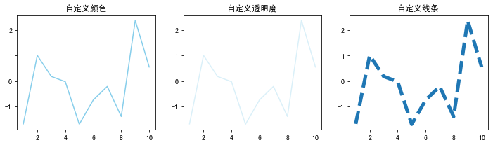

带注释的折线图

import matplotlib.pyplot as plt
import numpy as np
import pandas as pd

plt.rcParams['font.sans-serif'] = ['SimHei'] # 用来正常显示中文标签

# 自定义数据
dates = []

for date in range(1970,2023):
    dates.append(str(date))


sample_size = 2023-1970
variable = np.random.normal(100,
                            15,
                            sample_size,
                           )

df = pd.DataFrame({'date': dates,
                   'value': variable})


# 初始化布局
fig = plt.figure(figsize=(12,8))


# 1-基本折线图
plt.subplot(2, 1, 1) 
plt.plot(df['date'], df['value'])

# 轴标签
plt.xlabel('X-axis')
plt.ylabel('Y-axis')
plt.title('基本折线图')

# 刻度
plt.xticks(rotation=45)


# 2-带注释的折线图
plt.subplot(2, 1, 2) 
plt.plot(df['date'], df['value'])

# 轴标签
plt.xlabel('X-axis')
plt.ylabel('Y-axis')
plt.title('带注释的折线图')

# 刻度
plt.xticks(rotation=45)

# 添加文本注释
plt.text(df['date'].iloc[38], # x位置
         df['value'].iloc[1], # y位置
         'What a nice chart!', # 文本注释
         fontsize=13,
         color='red')

# 找到最大值索引
highest_index = df['value'].idxmax()

# 最高值标记
plt.scatter(df['date'].iloc[highest_index],
            df['value'].iloc[highest_index],
            color='blue',
            marker='o', # 标记特殊的店
            s=100,
           )

# 计算均值
median_value = df['value'].median()

# 添加均值线
plt.axhline(y=median_value, color='green', linestyle='--', label='Reference Line (Median)')


fig.tight_layout() # 自动调整间距
plt.show()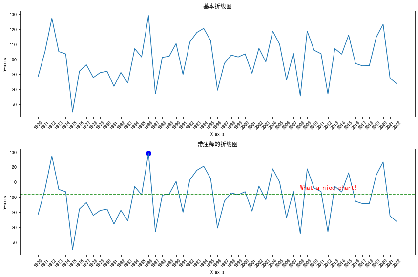

对数变换的折线图

import matplotlib.pyplot as plt
from matplotlib.ticker import MultipleLocator
import numpy as np
import pandas as pd

plt.rcParams['font.sans-serif'] = ['SimHei'] # 用来正常显示中文标签

# 自定义数据
x = np.linspace(1, 10, 100)
y = np.exp(x)
df = pd.DataFrame({'x': x, 'y': y})

# 初始化布局
fig = plt.figure(figsize=(12,4))


# 1-基本折线图
plt.subplot(1, 2, 1) 
plt.plot(df['x'], df['y'])

# 轴标签
plt.xlabel('X-axis')
plt.ylabel('Y-axis')
plt.title('基本折线图')

# 添加网格线
plt.grid(True, linestyle='--', alpha=0.6)

# 2-对数转化折线图
plt.subplot(1, 2, 2) 
plt.plot(df['x'], df['y'])

# y轴对数化
plt.yscale('log')

# 轴标签
plt.xlabel('X-axis')
plt.ylabel('Y-axis')
plt.title('对数化的折线图')

# 对数刻度的网格
y_major_locator = MultipleLocator(3000) 
plt.gca().yaxis.set_major_locator(y_major_locator)

# 添加网格线
plt.grid(True, linestyle='--', alpha=0.6)

plt.show()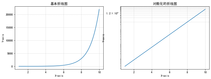

双轴折线图

import matplotlib.pyplot as plt
import numpy as np
from datetime import datetime, timedelta
from matplotlib import colors

plt.rcParams['font.sans-serif'] = ['SimHei'] # 用来正常显示中文标签

rng = np.random.default_rng(1234)

date = [datetime(2019, 1, 1) + timedelta(i) for i in range(100)]
temperature = np.arange(100) ** 2.5 / 10000 + rng.uniform(size=100)
price = np.arange(120, 20, -1) ** 1.5 / 10 + rng.uniform(size=100)

# 设置多子图
fig, axarr = plt.subplots(2, 2, figsize=(12, 8))

# 1-基础的双轴折线图
ax1 = axarr[0, 0]
ax2 = ax1.twinx()
ax1.plot(date, temperature)
ax2.plot(date, price)
ax1.set_title('基础的双轴折线图')

# 2-自定义颜色双轴
COLOR_TEMPERATURE = "#69b3a2"
COLOR_PRICE = "#3399e6"

ax1 = axarr[0, 1]
ax2 = ax1.twinx()
ax1.plot(date, temperature, color=COLOR_TEMPERATURE, lw=3)
ax2.plot(date, price, color=COLOR_PRICE, lw=4)

ax1.set_xlabel("Date")
ax1.set_ylabel("Temperature (Celsius °)", color=COLOR_TEMPERATURE, fontsize=14)
ax1.tick_params(axis="y", labelcolor=COLOR_TEMPERATURE)
ax2.set_ylabel("Price ($)", color=COLOR_PRICE, fontsize=14)
ax2.tick_params(axis="y", labelcolor=COLOR_PRICE)
ax1.set_title('自定义颜色双轴')

# 3-折线与条形图组合
ax1 = axarr[1, 0]
ax2 = ax1.twinx()
ax1.bar(date, temperature, color=COLOR_TEMPERATURE, edgecolor="black", alpha=0.4, width=1.0)
ax2.plot(date, price, color=COLOR_PRICE, lw=4)

ax1.set_xlabel("Date")
ax1.set_ylabel("Temperature (Celsius °)", color=COLOR_TEMPERATURE, fontsize=14)
ax1.tick_params(axis="y", labelcolor=COLOR_TEMPERATURE)

ax2.set_ylabel("Price ($)", color=COLOR_PRICE, fontsize=14)
ax2.tick_params(axis="y", labelcolor=COLOR_PRICE)

fig.autofmt_xdate()
ax1.set_title("折线与条形图组合")

# 4-自定义组合图样式
color = list(colors.to_rgba(COLOR_TEMPERATURE))
color[3] = 0.4

ax1 = axarr[1, 1]
ax2 = ax1.twinx()
ax1.bar(date, temperature, color=color, edgecolor="black", width=1.0)
ax2.plot(date, price, color=COLOR_PRICE, lw=4)

ax1.set_xlabel("Date")
ax1.set_ylabel("Temperature (Celsius °)", color=COLOR_TEMPERATURE, fontsize=14)
ax1.tick_params(axis="y", labelcolor=COLOR_TEMPERATURE)

ax2.set_ylabel("Price ($)", color=COLOR_PRICE, fontsize=14)
ax2.tick_params(axis="y", labelcolor=COLOR_PRICE)

fig.autofmt_xdate()
ax1.set_title("自定义组合图样式")


fig.tight_layout() # 自动调整间距
plt.show()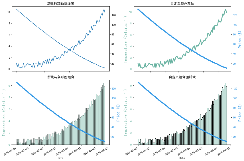

多个折线图

import matplotlib.pyplot as plt
import numpy as np
from datetime import datetime, timedelta
from matplotlib import colors
import matplotlib.gridspec as gridspec

plt.rcParams['font.sans-serif'] = ['SimHei'] # 用来正常显示中文标签

# 创建 2x3 的大布局
fig = plt.figure(figsize=(18, 8))
gs = gridspec.GridSpec(2, 3, figure=fig)
# 获得每个子图的位置
ax1 = fig.add_subplot(gs[0, 0])
ax2 = fig.add_subplot(gs[0, 1])
ax3 = fig.add_subplot(gs[0, 2])
# ax4 = fig.add_subplot(gs[1, 0])
# ax5 = fig.add_subplot(gs[1, 1])
ax6 = fig.add_subplot(gs[1, 2])

# 1-基础的多折线图
df=pd.DataFrame({'x_values': range(1,11), 'y1_values': np.random.randn(10), 'y2_values': np.random.randn(10)+range(1,11), 'y3_values': np.random.randn(10)+range(11,21) })

ax1.plot( 'x_values', 'y1_values', data=df, marker='o', markerfacecolor='blue', markersize=12, color='skyblue', linewidth=4)
ax1.plot( 'x_values', 'y2_values', data=df, marker='', color='olive', linewidth=2)
ax1.plot( 'x_values', 'y3_values', data=df, marker='', color='olive', linewidth=2, linestyle='dashed', label="toto")
ax1.legend()
ax1.set_title('基础的多折线图')



# 2-高亮显示一组
df=pd.DataFrame({'x': range(1,11), 'y1': np.random.randn(10), 'y2': np.random.randn(10)+range(1,11), 'y3': np.random.randn(10)+range(11,21), 'y4': np.random.randn(10)+range(6,16), 'y5': np.random.randn(10)+range(4,14)+(0,0,0,0,0,0,0,-3,-8,-6), 'y6': np.random.randn(10)+range(2,12), 'y7': np.random.randn(10)+range(5,15), 'y8': np.random.randn(10)+range(4,14) })

for column in df.drop('x', axis=1):
    ax2.plot(df['x'], df[column], marker='', color='grey', linewidth=1, alpha=0.4)
ax2.plot(df['x'], df['y5'], marker='', color='orange', linewidth=4, alpha=0.7) # 高亮y5
ax2.set_xlim(0,12)
# 增加注释
num=0
for i in df.values[9][1:]:
    num+=1
    name=list(df)[num]
    if name != 'y5':
        ax2.text(10.2, i, name, horizontalalignment='left', size='small', color='grey')
    else:
        ax2.text(10.2, i, 'Mr Orange', horizontalalignment='left', size='small', color='orange') # 高亮组的文本注释
ax2.set_title("高亮显示一组")



# 3-多折线模式（Spaghetti Plot）
df=pd.DataFrame({'x': range(1,11), 'y1': np.random.randn(10), 'y2': np.random.randn(10)+range(1,11), 'y3': np.random.randn(10)+range(11,21), 'y4': np.random.randn(10)+range(6,16), 'y5': np.random.randn(10)+range(4,14)+(0,0,0,0,0,0,0,-3,-8,-6), 'y6': np.random.randn(10)+range(2,12), 'y7': np.random.randn(10)+range(5,15), 'y8': np.random.randn(10)+range(4,14), 'y9': np.random.randn(10)+range(4,14), 'y10': np.random.randn(10)+range(2,12) })

palette = plt.get_cmap('Set1')
num=0
for column in df.drop('x', axis=1):
    num+=1
    ax3.plot(df['x'], df[column], marker='', color=palette(num), linewidth=1, alpha=0.9, label=column)
    
ax3.legend(loc=2, ncol=2)
ax3.set_title("多折线模式（Spaghetti Plot）")



# 4-多折线小图
df=pd.DataFrame({'x': range(1,11), 'y1': np.random.randn(10), 'y2': np.random.randn(10)+range(1,11), 'y3': np.random.randn(10)+range(11,21), 'y4': np.random.randn(10)+range(6,16), 'y5': np.random.randn(10)+range(4,14)+(0,0,0,0,0,0,0,-3,-8,-6), 'y6': np.random.randn(10)+range(2,12), 'y7': np.random.randn(10)+range(5,15), 'y8': np.random.randn(10)+range(4,14), 'y9': np.random.randn(10)+range(4,14) })
# 在第一行第一列的位置创建3*3的子布局
ax4 = gridspec.GridSpecFromSubplotSpec(3, 3, subplot_spec=gs[1, 0])
# 在 3x3 的小布局中添加子图
axes = []
for i in range(3):
    for j in range(3):
        ax = fig.add_subplot(ax4[i, j])
        axes.append(ax)  # 将子图句柄添加到列表中
num = 0
for column in df.drop('x', axis=1):
    num += 1

    ax = axes[num - 1]
    ax.plot(df['x'], df[column], marker='', color=palette(num), linewidth=1.9, alpha=0.9, label=column)
    ax.set_xlim(0,10)
    ax.set_ylim(-2,22)


    # 如果当前子图不在最左边，就不显示y轴的刻度标签
    if num not in [1,4,7] :
        ax.tick_params(labelleft=False)
        
    # 如果当前子图不在最下边，就不显示x轴的刻度标签
    if num not in [7,8,9] :
        ax.tick_params(labelbottom=False)
        
    ax.annotate(column, xy=(0, 1), xycoords='axes fraction', fontsize=12, fontweight=0, color=palette(num),
            xytext=(5, -5), textcoords='offset points', ha='left', va='top')
    
axes[1].set_title('多折线小图') # 通过设置3*3图的第二个子图的标题替代2*3图中的第4个图的子标题
    
    
# 5-多折线小图细节处理
df=pd.DataFrame({'x': range(1,11), 'y1': np.random.randn(10), 'y2': np.random.randn(10)+range(1,11), 'y3': np.random.randn(10)+range(11,21), 'y4': np.random.randn(10)+range(6,16), 'y5': np.random.randn(10)+range(4,14)+(0,0,0,0,0,0,0,-3,-8,-6), 'y6': np.random.randn(10)+range(2,12), 'y7': np.random.randn(10)+range(5,15), 'y8': np.random.randn(10)+range(4,14), 'y9': np.random.randn(10)+range(4,14) })
# 在第一行第一列的位置创建3*3的子布局
ax5 = gridspec.GridSpecFromSubplotSpec(3, 3, subplot_spec=gs[1, 1])
# 在 3x3 的小布局中添加子图
axes = []
for i in range(3):
    for j in range(3):
        ax = fig.add_subplot(ax5[i, j])
        axes.append(ax)  # 将子图句柄添加到列表中
num=0
for column in df.drop('x', axis=1):
    num+=1
 
    ax = axes[num - 1]
    for v in df.drop('x', axis=1):
        ax.plot(df['x'], df[v], marker='', color='grey', linewidth=0.6, alpha=0.3)
 
    ax.plot(df['x'], df[column], marker='', color=palette(num), linewidth=2.4, alpha=0.9, label=column)
 
    ax.set_xlim(0,10)
    ax.set_ylim(-2,22)
 
     # 如果当前子图不在最左边，就不显示y轴的刻度标签
    if num not in [1,4,7] :
        ax.tick_params(labelleft=False)
        
    # 如果当前子图不在最下边，就不显示x轴的刻度标签
    if num not in [7,8,9] :
        ax.tick_params(labelbottom=False)
        
    ax.annotate(column, xy=(0, 1), xycoords='axes fraction', fontsize=12, fontweight=0, color=palette(num),
            xytext=(5, -5), textcoords='offset points', ha='left', va='top')
    
axes[1].set_title('多折线小图细节处理') # 通过设置3*3图的第二个子图的标题替代2*3图中的第5个图的子标题
    
    
# 6-带区域填充的多折线图
time = np.arange(12)
income = np.array([5, 9, 6, 6, 10, 7, 6, 4, 4, 5, 6, 4])
expenses = np.array([6, 6, 8, 3, 6, 9, 7, 8, 6, 6, 4, 8])

ax6.plot(time, income, color="green")
ax6.plot(time, expenses, color="red")

# 当income > expenses填充绿色
ax6.fill_between(
    time, income, expenses, where=(income > expenses), 
    interpolate=True, color="green", alpha=0.25, 
    label="Positive"
)

# 当income <= expenses填充红色
ax6.fill_between(
    time, income, expenses, where=(income <= expenses), 
    interpolate=True, color="red", alpha=0.25,
    label="Negative"
)

ax6.set_title('带区域填充的多折线图')
ax6.legend()


plt.tight_layout() # 自动调整间距
plt.show()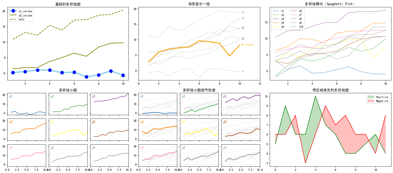

绘制时间序列图

import matplotlib.pyplot as plt
import pandas as pd
import matplotlib.dates as mdates

# 导入数据
data = pd.read_csv(
    "https://raw.githubusercontent.com/holtzy/data_to_viz/master/Example_dataset/3_TwoNumOrdered.csv", 
    delim_whitespace=True
)

# 日期格式
data["date"] = pd.to_datetime(data["date"])

date = data["date"]
value = data["value"]

# 绘制时间序列图
fig, ax = plt.subplots(figsize=(8, 6))

# 设置6个月间隔为一刻度
half_year_locator = mdates.MonthLocator(interval=6) # 半年刻度
monthly_locator = mdates.MonthLocator() # 每月子刻度
year_month_formatter = mdates.DateFormatter("%Y-%m") # 格式化日期yyyy-MM

ax.xaxis.set_major_locator(half_year_locator)
ax.xaxis.set_minor_locator(monthly_locator)
ax.xaxis.set_major_formatter(year_month_formatter)

ax.plot(date, value)

fig.autofmt_xdate() # 自动旋转轴标签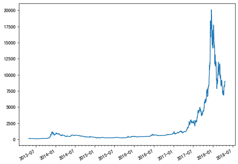

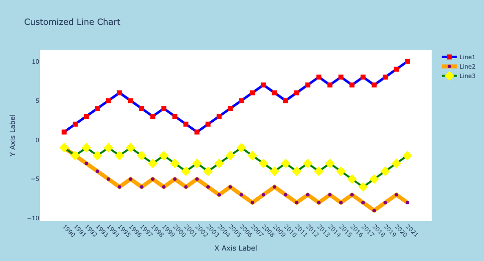
通过plotly绘制多样化的折线图

import plotly.graph_objects as go
import numpy as np
import pandas as pd

# 自定义数据

dates = []
start = 1990
end = 2022
for date in range(start,end):
    dates.append(str(date))
    
# 生成随机序列，并计算累计和来生成随机漫步1、2、3
random_steps = np.random.choice([-1, 1], size=end-start, p=[0.5, 0.5])
random_walk1 = np.cumsum(random_steps)

random_steps = np.random.choice([-1, 1], size=end-start, p=[0.5, 0.5])
random_walk2 = np.cumsum(random_steps)

random_steps = np.random.choice([-1, 1], size=end-start, p=[0.5, 0.5])
random_walk3 = np.cumsum(random_steps)

# 具有三个随机漫步的数据
df = pd.DataFrame({'date': dates,
                   'value1': random_walk1,
                   'value2': random_walk2,
                   'value3': random_walk3,})


fig = go.Figure()

# 自定义变量1
fig.add_trace(go.Scatter(
    x=df['date'],
    y=df['value1'],
    mode='lines+markers', # 点线连接样式
    name='Line1',
    
    marker=dict(
        symbol='square',    
        size=10,           
        color='red'),      
    
    line=dict(
        color='blue',        
        width=5)            
))

# 自定义变量2
fig.add_trace(go.Scatter(
    x=df['date'], 
    y=df['value2'], 
    mode='lines+markers', 
    name='Line2', 
    
    marker=dict(
        symbol='circle',   
        size=7,           
        color='purple'),      
    
    line=dict(
        color='orange',       
        width=8)            
))

# 自定义变量3
fig.add_trace(go.Scatter(
    x=df['date'], 
    y=df['value3'], 
    mode='lines+markers', 
    name='Line3',
    
    marker=dict(
        symbol='diamond',    
        size=15,            
        color='yellow'),       
    
    line=dict(
        color='green',       
        width=4)             
))

# 自定义布局
fig.update_layout(
    title='Customized Line Chart',
    xaxis_title='X Axis Label', 
    yaxis_title='Y Axis Label',
    xaxis_tickangle=45,  
    showlegend=True,    
    plot_bgcolor='white',  
    paper_bgcolor='lightblue', 
)

通过pandas绘制多样化的折线图

修改参数

import pandas as pd
import matplotlib.pyplot as plt


# 导入数据
url = 'https://raw.githubusercontent.com/holtzy/The-Python-Graph-Gallery/master/static/data/gapminderData.csv'
df = pd.read_csv(url)
df_france = df[df['country']=='France']


# 绘制折线图
ax = df_france.plot(x='year',
                    y='lifeExp',
                    grid=True,
                    linestyle='--',
                    alpha=0.5,
                    color='purple',
                    linewidth=2.0, 
                    marker='d',  
                    markersize=8,  
                    markerfacecolor='orange', 
                    label='France'
                   )

# 标题
ax.set_title('Evolution of \nthe life expectancy in France',
             weight='bold') 

# 轴标签
ax.set_ylabel('Life Expectancy')
ax.set_xlabel('Time (in year)')


plt.show()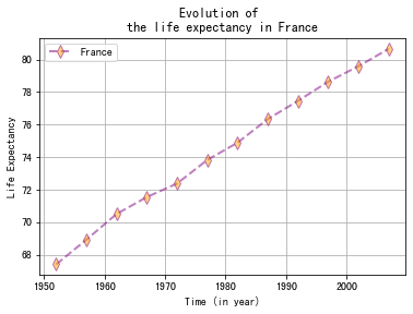

多变量折线图

import pandas as pd
import random, numpy as np
import matplotlib.pyplot as plt

# 自定义数据
num_time_points = 100
time_values = np.arange(num_time_points)

temperature = np.random.uniform(200, 400, num_time_points) 
pressure = np.random.uniform(500, 700, num_time_points) 
humidity = np.random.uniform(800, 1000, num_time_points) 

data = {
    'Time': time_values,
    'Temperature': temperature,
    'Pressure': pressure,
    'Humidity': humidity
}
df = pd.DataFrame(data)

# 绘制多变量折线图
df.plot(x='Time',
        kind='line', 
        grid=True, 
        )
plt.legend(loc='upper right',
           bbox_to_anchor=(1.35, 1), 
          )
plt.show()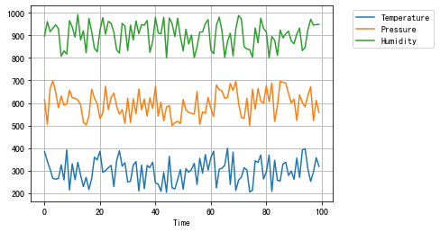

分组折线图

import pandas as pd
import random, numpy as np
import matplotlib.pyplot as plt

# 自定义数据
num_data_points_per_country = 20

# 设置多个国家的温度
france_temperatures = np.random.uniform(10, 20, num_data_points_per_country)  
germany_temperatures = np.random.uniform(0, 10, num_data_points_per_country) 
italy_temperatures = np.random.uniform(25, 30, num_data_points_per_country) 

# 对应的国家数据
countries = ['France', 'Germany', 'Italy']
country_labels = np.repeat(countries, num_data_points_per_country)

# 时间数据
time_values = np.tile(np.arange(num_data_points_per_country), len(countries))

data = {
    'Country': country_labels,
    'Temperature': np.concatenate([france_temperatures, germany_temperatures, italy_temperatures]),
    'Time': time_values
}

df = pd.DataFrame(data)


# 绘制折线图
for name, group in df.groupby('Country'):
    plt.plot(group['Time'], group['Temperature'], label=name)

# 设置图表的标题和坐标轴标签，并显示图例
plt.title('Temperature Trend over Time by Country')
plt.xlabel('Time')
plt.ylabel('Temperature')
plt.legend(bbox_to_anchor=(1.05, 1), loc='upper left')

# 显示图表
plt.show()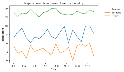

总结

以上通过matplotlib、seaborn、plotly和pandas快速绘制折线图。并通过修改参数或者辅以其他绘图知识自定义各种各样的折线图来适应相关使用场景。

共勉～

原文地址：https://blog.csdn.net/weixin_39293132/article/details/142920341

免责声明：本站文章内容转载自网络资源，如本站内容侵犯了原著者的合法权益，可联系本站删除。更多内容请关注自学内容网（zxcms.com）！

上一篇：条款7 区分使用( )和{ }
下一篇：PDA手持终端一步到位的扫码解决方案

leetcode289:生命游戏
根据，简称为，是英国数学家约翰·何顿·康威在 1970 年发明的细胞自动机。给定一个包含m × n个格子的面板，每一个格子都可以看成是一个细胞。每个细胞都具有一个初始状态：1即为（live），或0即为
阅读更多2024-10-20
MongoDB数据恢复
注意：两个MongoDB的版本要一致，本文使用的是mongo:4.2.24。先把K8S上面的MongoDB 容器停止（可以把副本改成0）。1、将容器挂载MongoDB的数据目录备份到本地。经常是数据文
阅读更多2024-10-20
C#中实现事务
C#中实现事务
阅读更多2024-10-20
【LeetCode每日一题】——560.和为 K 的子数组
给你一个整数数组 nums 和一个整数 k ，请你统计并返回该数组中和为 k 的子数组的个数。子数组是数组中元素的连续非空序列。
阅读更多2024-10-20
「漏洞复现」满客宝智慧食堂系统 selectUserByOrgId 未授权访问漏洞
请勿利用文章内的相关技术从事非法测试，由于传播、利用此文所提供的信息而造成的任何直接或者间接的后果及损失，均由使用者本人负责，作者不为此承担任何责任。工具来自网络，安全性自测，如有侵权请联系删除。本次
阅读更多2024-10-20
React面试题目（从基本到高级）
React前端面试常见题目涵盖了React的基础概念、组件、状态管理、生命周期、性能优化等多个方面。
阅读更多2024-10-20
12.个人博客系统（Java项目基于spring和vue）
1 在校学习的学生，可用于日常学习使用或是毕业设计使用 2 毕业一到两年的开发人员，用于锻炼自己的独立功能模块设计能力，增强代码编写能力。 3 亦可以部署为商化项目使用。 4 需要完整资料及源码
阅读更多2024-10-20
YoloV8改进策略：注意力改进|DeBiFormer，可变形双级路由注意力|引入DeBiLevelRoutingAttention注意力模块（全网首发）
本次改进的核心在于将DeBiLevelRoutingAttention模块嵌入到YoloV8的主干网络中，具体位置是在SPPF（Spatial Pyramid Pooling Fast）模块之后。这一
阅读更多2024-10-20
word取消自动单词首字母大写
情况说明：在word输入单词后首字母会自动变成大写取消单词首字母大写步骤：（1）点击菜单栏文件（2）点击“更多”——>“选项”（3）点击“校对”——>“自动更正选项”（4）取消“句首字母大
阅读更多2024-10-20
web前端网页用户注册页面
【代码】web前端网页用户注册页面。
阅读更多2024-10-20

趋势（一）利用python绘制折线图

趋势（一）利用python绘制折线图

折线图（ Line Chart）简介

快速绘制

定制多样化的折线图

通过matplotlib绘制多样化的折线图

通过plotly绘制多样化的折线图

通过pandas绘制多样化的折线图

总结

相关文章