从0开始深度学习（12）——多层感知机的逐步实现

依然以Fashion-MNIST图像分类数据集为例，手动实现多层感知机和激活函数的编写，大部分代码均在从0开始深度学习（9）——softmax回归的逐步实现中实现过

1 读取数据

import torch
from torchvision import transforms
import torchvision
from torch.utils import data

# 读取数据
def load_data_fashion_mnist(batch_size, resize=None):  #@save
    trans = [transforms.ToTensor()]
    if resize:
        trans.insert(0, transforms.Resize(resize))
    trans = transforms.Compose(trans)
    mnist_train = torchvision.datasets.FashionMNIST(
        root="D:/DL_Data/", train=True, transform=trans, download=False)
    mnist_test = torchvision.datasets.FashionMNIST(
        root="D:/DL_Data/", train=False, transform=trans, download=False)
    return (data.DataLoader(mnist_train, batch_size, shuffle=True,
                            num_workers=12),
            data.DataLoader(mnist_test, batch_size, shuffle=False,
                            num_workers=12))
                            
train_iter, test_iter = load_data_fashion_mnist(256, resize=28)

2 初始化模型参数

以单隐藏层的多层感知机为例，选择使用256个隐藏单元

from torch import nn

# 初始化模型参数
num_inputs=784      # 28*28
num_outputs=10
num_hiddens=256     # 我们选择使用256个隐藏单元，注意，一般选择使用2的若干次幂，因为内存的特殊性，可以在计算上更高效

w1 = nn.Parameter(torch.randn(num_inputs,num_hiddens,requires_grad=True)*0.01)
b1 = nn.Parameter(torch.zeros(num_hiddens,requires_grad=True))

w2 = nn.Parameter(torch.randn(num_hiddens, num_outputs, requires_grad=True) * 0.01)
b2 = nn.Parameter(torch.zeros(num_outputs, requires_grad=True))

params = [w1, b1, w2, b2]

3 激活函数、损失函数、建立模型

# 激活函数
def relu(x):
    a=torch.zeros_like(x) # 保证全零张量和x的形状一致，利于广播计算
    return torch.max(x,a)

# 损失函数
loss = nn.CrossEntropyLoss(reduction='none')

#建立模型
def net(x):
    x=x.reshape((-1,num_inputs))#展开
    H=relu(x@w1+b1)# @表示矩阵乘法
    return (H@w2+b2)

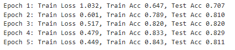
4 训练模型

优化器使用SGD

#训练，优化器使用sgd
num_epochs=5
lr=00.1
updater=torch.optim.SGD(params,lr=lr)

def train_epoch(net, train_iter, loss, updater):
    if isinstance(net, torch.nn.Module):
        net.train()  # 将模型设置为训练模式
    metric = Accumulator(3)  # 训练损失总和、训练准确度总和、样本数
    for X, y in train_iter:
        y_hat = net(X)
        l = loss(y_hat, y).mean()
        if isinstance(updater, torch.optim.Optimizer):
            updater.zero_grad()
            l.backward()
            updater.step()
        else:
            l.backward()
            updater([w, b], lr, batch_size)
        metric.add(float(l) * y.numel(), compute_accuracy(y_hat, y), y.numel())
    return metric[0] / metric[2], metric[1] / metric[2]

def train(net, train_iter, test_iter, loss, num_epochs, updater):
    for epoch in range(num_epochs):
        train_metrics = train_epoch(net, train_iter, loss, updater)
        test_acc = evaluate_accuracy(net, test_iter)
        print(f'Epoch {epoch + 1}: Train Loss {train_metrics[0]:.3f}, Train Acc {train_metrics[1]:.3f}, Test Acc {test_acc:.3f}')
        
class Accumulator:  #@save
    """在n个变量上累加"""
    def __init__(self, n):
        self.data = [0.0] * n

    def add(self, *args):
        self.data = [a + float(b) for a, b in zip(self.data, args)]

    def reset(self):
        self.data = [0.0] * len(self.data)

    def __getitem__(self, idx):
        return self.data[idx]

def compute_accuracy(y_hat, y):  # 预测值、真实值
    if len(y_hat.shape) > 1 and y_hat.shape[1] > 1:
        y_hat = y_hat.argmax(axis=1)  # 找到一个样本中，对应的最大概率的类别
    cmp = y_hat.type(y.dtype) == y  # 将预测值 y_hat 与真实标签 y 进行比较，生成一个布尔张量 cmp
    return float(cmp.type(y.dtype).sum())

# 计算在指定数据集上模型的准确率
def evaluate_accuracy(net, data_iter):  
    if isinstance(net, torch.nn.Module):
        net.eval()  # 将模型设置为评估模式
    metric = Accumulator(2)  # 累加多个变量的总和。这里初始化了一个包含两个元素的累加器，分别用来存储正确预测的数量和总的预测数量。
    with torch.no_grad():
        for X, y in data_iter:
            metric.add(compute_accuracy(net(X), y), y.numel())
    return metric[0] / metric[1]

train(net, train_iter, test_iter, loss, num_epochs, updater)

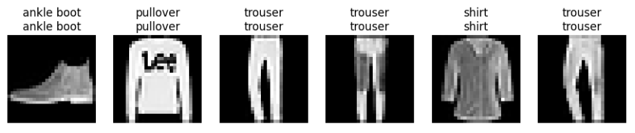
5 预测

import matplotlib.pyplot as plt
# 定义 Fashion-MNIST 标签的文本描述
def get_fashion_mnist_labels(labels):
    text_labels = ['t-shirt', 'trouser', 'pullover', 'dress', 'coat',
                   'sandal', 'shirt', 'sneaker', 'bag', 'ankle boot']
    return [text_labels[int(i)] for i in labels]

# 预测并显示结果
def predict(net, test_iter, n=6):
    for X, y in test_iter:
        break  # 只取一个批次的数据
    trues = get_fashion_mnist_labels(y)
    preds = get_fashion_mnist_labels(net(X).argmax(axis=1))
    titles = [true + '\n' + pred for true, pred in zip(trues, preds)]
    n = min(n, X.shape[0])
    fig, axs = plt.subplots(1, n, figsize=(12, 3))
    for i in range(n):
        axs[i].imshow(X[i].permute(1, 2, 0).squeeze().numpy(), cmap='gray')
        axs[i].set_title(titles[i])
        axs[i].axis('off')
    plt.show()

# 调用预测函数
predict(net, test_iter, n=6)

原文地址：https://blog.csdn.net/m0_53115174/article/details/143020820

免责声明：本站文章内容转载自网络资源，如本站内容侵犯了原著者的合法权益，可联系本站删除。更多内容请关注自学内容网（zxcms.com）！