Coursera吴恩达机器学习专项课程02：Advanced Learning Algorithms 笔记 Week04 （完结）

Week 04 of Advanced Learning Algorithms

笔者在2022年7月份取得这门课的证书，现在（2024年2月25日）才想起来将笔记发布到博客上。

Website: https://www.coursera.org/learn/advanced-learning-algorithms?specialization=machine-learning-introduction

Offered by: DeepLearning.AI and Stanford

课程地址：https://www.coursera.org/learn/machine-learning

本笔记包含字幕，quiz的答案以及作业的代码，仅供个人学习使用，如有侵权，请联系删除。

This week, you’ll learn about a practical and very commonly used learning algorithm the decision tree. You’ll also learn about variations of the decision tree, including random forests and boosted trees (XGBoost).

Learning Objectives

---

• See what a decision tree looks like and how it can be used to make predictions
• Learn how a decision tree learns from training data
• Learn the “impurity” metric “entropy” and how it’s used when building a decision tree
• Learn how to use multiple trees, “tree ensembles” such as random forests and boosted trees
• Learn when to use decision trees or neural networks

[1] Decision trees

Decision tree model

Ear shape: pointy, floppy

Face shape: round, not round

Whiskers: present, not absent

Welcome to the final week of this course on Advanced
Learning Algorithms.

One to the learning
algorithm is this very powerful why we use
many applications, also used by many to win machine learning competitions is decision trees and
tree ensembles.

Despite all the successes
of decision trees, they somehow haven’t received that much attention in academia, and so you may not hear about decision trees nearly that much, but it is a tool well worth
having in your toolbox.

In this week, we’ll learn about decision trees
and you’ll see how to get them to work for
yourself.

Let’s dive in.

To explain how
decision trees work, I’m going to use as a
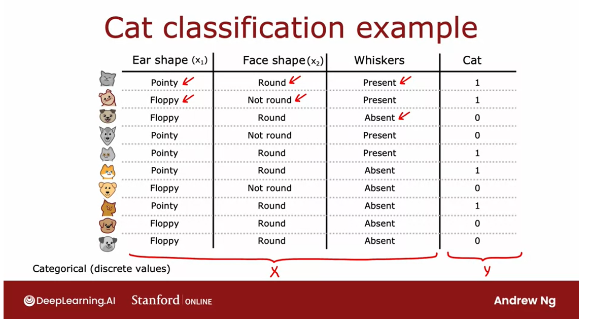
running example this week a cat classification example.

Train a classifier to quickly tell you if an animal is a cat or not

You are running a
cat adoption center and given a few features, you want to train
a classifier to quickly tell you if an
animal is a cat or not.

I have here 10
training examples.

Associated with each
of these 10 examples, we’re going to have features regarding the
animal’s ear shape, face shape, whether
it has whiskers, and then the ground truth
label that you want to predict this animal cat.

The first example
has pointy ears, round face, whiskers are
present, and it is a cat.

The second example
has floppy ears, the face shape is not round, whiskers are present, and yes, that is a cat, and so on for
the rest of the examples.

This dataset has five
cats and five dogs in it. The input features X are
these three columns, and the target output
that you want to predict, Y, is this final column of, is this a cat or not?

In this example, the features X take on categorical values.

In other words, the
features take on just a few discrete values. Your shapes are either
pointy or floppy.

The face shape is either
round or not round and whiskers are either
present or absent.

This is a binary
classification task because the labels
are also one or zero.

For now, each of
the features X_1, X_2, and X_3 take on only
two possible values.

We’ll talk about
features that can take on more than
two possible values, as well as continuous-valued
features later in this week. What is a decision tree?

What is a decision tree?

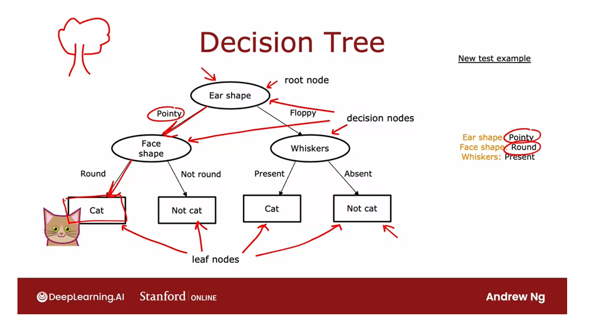
Here’s an example of a model
that you might get after training a decision
tree learning algorithm on the data
set that you just saw.

The model that is output by the learning algorithm
looks like a tree, and a picture like this is what computer scientists call a tree.

If it looks nothing like the biological trees that
you see out there to you, it’s okay, don’t worry about it.

We’ll go through an
example to make sure that this computer science
definition of a tree makes sense
to you as well.

Every one of these ovals or rectangles is called
a node in the tree.

If you haven’t seen computer scientists’
definitions of trees before, it may seem non-intuitive
that the roots of the tree is at the top and the leaves of the tree are down at the bottom.

Maybe one way to
think about this is this is more akin to an
indoor hanging plant, which is why the
roots are up top, and then the leaves tend to fall down to the
bottom of the tree.

The way this model works is if you have a new test example, she has a cat where the
ear-shaped has pointy, face shape is round, and
whiskers are present.

The way this model will look at this example and make a
classification decision is will start with this example at this
topmost node of the tree, this is called the
root node of the tree, and we will look at the feature written inside,
which is ear shape.

Based on the value of the
ear shape of this example we’ll either go
left or go right.

The value of the ear-shape
with this example is pointy, and so we’ll go down the
left branch of the tree, like so, and end up at
this oval node over here.

We then look at the face
shape of this example, which turns out to be round, and so we will follow this
arrow down over here.

The algorithm will make a inference that it
thinks this is a cat.

You get to this node
and the algorithm will make a prediction
that this is a cat.

What I’ve shown on this slide is one specific
decision tree model.

The root node

To introduce a bit
more terminology, this top-most node in the
tree is called the root node.

Decision node: intermediate node

All of these nodes, that is, all of
these oval shapes, but excluding the
boxes at the bottom, all of these are
called decision nodes.

They’re decision nodes
because they look at a particular feature and then based on the
value of the feature, cause you to decide whether to go left or right down the tree.

Leaf node: rectangular boxes, nodes at the bottom

Finally, these nodes
at the bottom, these rectangular boxes
are called leaf nodes.

They make a prediction.

We’ll start at this
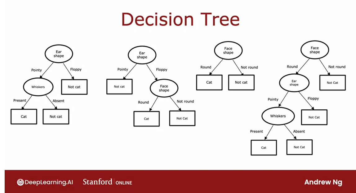
node here at the top. In this slide, I’ve shown just one example of
a decision tree. Here are a few others.

This is a different
decision tree for trying to classify cat versus not cat. In this tree, to make a
classification decision, you would again start at
this topmost root node.

Depending on their ear
shape of an example, you’d go either left or right.

If the ear shape is pointy, then you look at the
whiskers feature, and depending on whether
whiskers are present or absent, you go left or right to gain and classify cat versus not cat. Just for fun, here’s a second example of
a decision tree, here’s a third one, and here’s a fourth one.

Among these different
decision trees, some will do better and
some will do worse on the training sets or on the cross-validation
and test sets.

The job of the decision tree learning algorithm is, out of all possible decision trees, to try to pick one that hopefully does well on the training set, and then also ideally generalizes well to new data such as your cross-validation and test sets as well.

The job of the decision
tree learning algorithm is, out of all possible
decision trees, to try to pick one that hopefully does well
on the training set, and then also
ideally generalizes well to new data such as your cross-validation
and test sets as well.

Seems like there are lots of different decision trees one could build for a
given application. How do you get an
algorithm to learn a specific decision tree
based on a training set? Let’s take a look at
that in the next video.

Learning Process

The overall process of building a decision tree

The process of building a decision tree given a
training set has a few steps.

In this video, let’s
take a look at the overall process of what you need to do to
build a decision tree.

Given a training
set of 10 examples of cats and dogs like you
saw in the last video.

The first step: decide what feature to use at the root node

The first step of decision
tree learning is, we have to decide what feature
to use at the root node.

That is the first node at the very top of
the decision tree. [inaudible] algorithm that we’ll talk about in the
next few videos.

Let’s say that we decided to pick as the feature
and the root node, the ear shape feature.

What that means
is we will decide to look at all of our
training examples, all tangent examples shown here, I split them according to the value of the
ear shape feature.

In particular, let’s pick
out the five examples with pointy ears and move them
over down to the left.

Let’s pick the
five examples with floppy ears and move
them down to the right.

The second step: focusing on the left branch of the decision tree

The second step is
focusing just on the left part or sometimes
called the left branch of the decision tree to decide what nodes
to put over there.

In particular, what
feature that we want to split on or what feature
do we want to use next. [inaudible] an
algorithm that again, we’ll talk about
later this week.

Let’s say you decide to use
the face shape feature there.

What we’ll do now is take
these five examples and split these five examples into two subsets based on their
value of the face shape.

We’ll take the four
examples out of these five with a round face shape and move them down to the left. The one example with a not round face shape and
move it down to the right.

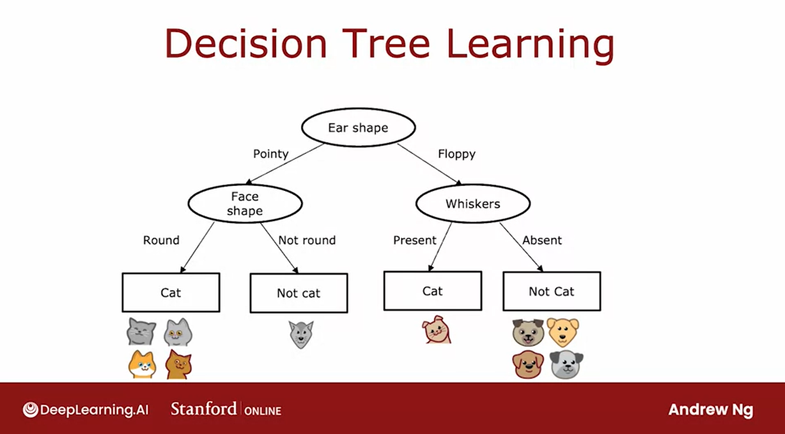
Finally, we notice that these four examples are all
cats four of them are cats.

Rather than splitting further, were created a leaf
node that makes a prediction that things that get down to that no other cats.

Over here we notice that none of the examples zero of
the one examples are cats or alternative 100 percent of the examples here are dogs.

We can create a
leaf node here that makes a prediction of not cat.

Repeat a similar process on the right branch of the decision tree.

Having done this on
the left part to the left branch of
this decision tree, we now repeat a
similar process on the right part or the right
branch of this decision tree.

Focus attention on just
these five examples, which contains one
captain for dogs. We would have to pick
some feature over here to use the split these
five examples further, if we end up choosing
the whiskers feature, we would then split these
five examples based on where the whiskers are
present or absent, like so.

You notice that one out of
one examples on the left for cats and zeros out
of four are cats.

Each of these nodes
is completely pure, meaning that is, all cats or not cats and there’s no longer
a mix of cats and dogs.

We can create these leaf nodes, making a cat
prediction on the left and a nightcap prediction
here on the right.

This is a process of
building a decision tree.

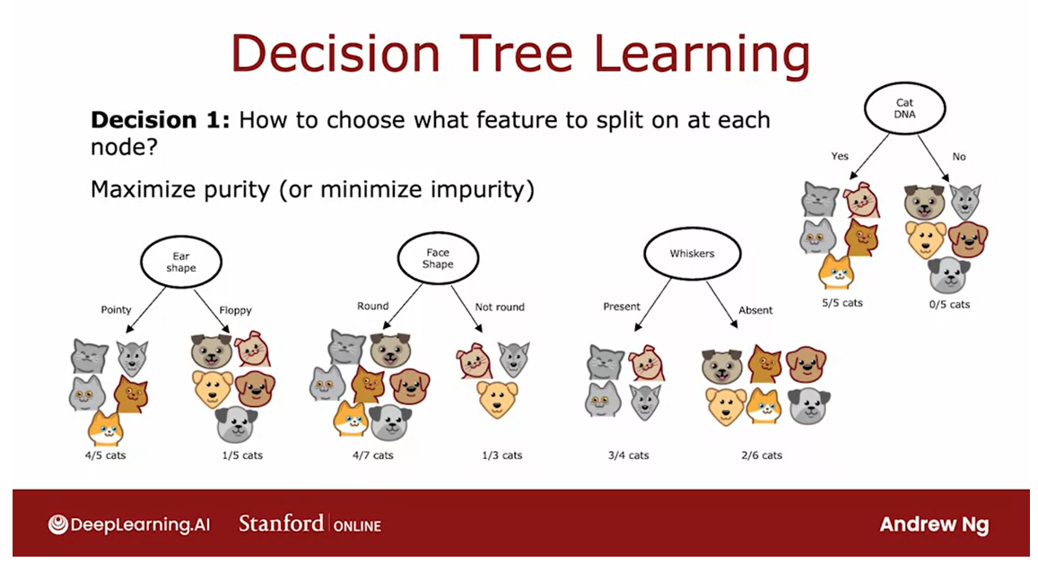
Decision 1: How to choose what feature to split on at each node?

A couple of key decisions that we had to make at various steps

Through this process, there were a couple of
key decisions that we had to make at various
steps during the algorithm.

Let’s talk through what those key decisions
were and we’ll keep on session of the details
of how to make these decisions in
the next few videos.

The first key decision was, how do you choose what features to use to
split on at each node?

At the root node, as well as on the left branch and the right branch of
the decision tree, we had to decide if there were a few examples at that node comprising a
mix of cats and dogs.

Max purity

Do you want to split on the ear-shaped feature or the facial feature or
the whiskers feature? We’ll see in the next video, that decision trees will
choose what feature to split on in order to try
to maximize purity.

By purity, I mean, you want to get to what subsets, which are as close as possible
to all cats or all dogs.

For example, if we had
a feature that said, does this animal have cat DNA, we don’t actually
have this feature.

But if we did, we could have split on this feature
at the root node, which would have
resulted in five out of five cats in the left branch and zero of the five cats
in the right branch.

Both these left and right subsets of the data
are completely pure, meaning that there’s
only one class, either cats only or not cats only in both of these left
and right sub-branches, which is why the cat DNA
feature if we had this feature, would have been a
great feature to use.

But with the features
that we actually have, we had to decide, what is the split on ear shape, which result in four out of five examples on the
left being cats, and one of the five examples on the right being cats or face shape where it resulted
in the four of the seven on the left and one
of the three on the right, or whiskers, which resulted
in three out four examples being cast on the
left and two out of six being not cats on the right.

The decision tree
learning algorithm has to choose between ear-shaped, face shape, and whiskers. Which of these
features results in the greatest purity of the labels on the left
and right sub branches?

Because it is if you can get to a highly pure
subsets of examples, then you can either predict cat or predict not cat
and get it mostly right.

The next video on entropy, we’ll talk about how to estimate impurity and how to
minimize impurity.

The first decision
we have to make when learning a decision tree is
how to choose which feature, the salon, and each node.

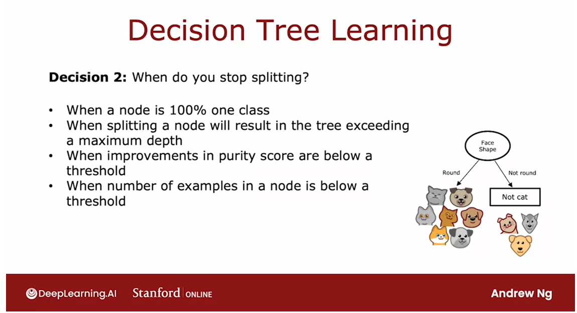
Decision 2: When do you stop splitting?

The second key decision you
need to make when building a decision tree is to decide
when do you stop splitting.

The criteria that
we use just now was until I know there’s
either 100 percent, all cats or a 100 percent
of dogs and not cats.

Because at that point is
seems natural to build a leaf node that just makes
a classification prediction.

Alternatively, you might also decide to stop splitting when splitting and no
further results in the tree exceeding
the maximum depth.

Where the maximum depth that you allow the
tree to go to, is a parameter that
you could just say.

Depth of a node

在决策树中，节点的深度定义为从表示为最顶端的根节点到该特定节点的跳数。

In decision tree, the depth of a node is
defined as the number of hops that it takes to get
from the root node that is denoted the very top
to that particular node.

So the root node
takes zero hops, it gets herself
and is at Depth 0. The notes below it
are at depth one and in those below it
would be at Depth 2.

If you had decided that the maximum depth of the
decision tree is say two, then you would decide not
to split any nodes below this level so that the tree
never gets to Depth 3.

By keeping the decision tree small, it makes it less prone to overfitting.

One reason you might want to limit the depth of
the decision tree is to make sure for
us to tree doesn’t get too big and
unwieldy and second, by keeping the tree small, it makes it less
prone to overfitting.

Another criteria you might
use to decide to stop splitting might be if the improvements in
the priority score, which you see in a later video of below
a certain threshold.

If splitting a node results
in minimum improvements to purity or you see later is actually decreases in impurity. But if the gains are too small, they might not bother.

Again, both to keep
the trees smaller and to reduce the
risk of overfitting.

If the number of examples that a node is below a certain threshold, then you might also decide to stop splitting.

Finally, if the number of examples that a node is
below a certain threshold, then you might also
decide to stop splitting.

For example, if at the root node we have split on the
face shape feature, then the right
branch will have had just three training
examples with one cat and two dogs and rather than splitting this into
even smaller subsets, if you decided not to split further sense of examples with just three
of your examples, then you will just create
a decision node and because there are maybe dogs
to other three adults here, this would be a
node and this makes a prediction of not cat.

Again, one reason you might
decide this is not worth splitting on is to keep the tree smaller and to
avoid overfitting.

When I look at
decision tree learning errands myself,
sometimes I feel like, boy, there’s a lot of
different pieces and lots of different things
going on in this algorithm.

Part of the reason it might feel is in the evolution
of decision trees.

There was one researcher that
proposed a basic version of decision trees and then a
different researcher said, oh, we can modify
this thing this way, such as his new
criteria for splitting.

Then a different researcher comes up with a different
thing like, oh, maybe we should stop sweating when it reaches a
certain maximum depth.

Over the years, different
researchers came up with different refinements
to the algorithm.

As a result of that, it does work really
well but we look at all the details of how
to implement a decision G. It feels a lot of
different pieces such as why there’s so many
different ways to decide when to stop splitting.

If it feels like a
somewhat complicated, messy average to you,
it does to me too.

But these different pieces, they do fit together into a very effective learning
algorithm and what you learn in this course is the key, most important ideas for
how to make it work well, and then at the
end of this week, I’ll also share with
you some guidance, some suggestions for how to use open source packages so that you don’t have to have
two complicates the procedure for making
all these decisions.

Like how do I decide
to stop splitting? You really get these atoms
to work well for yourself.

But I want to
reassure you that if this algorithm seems
complicated and messy, it frankly does to me too, but it does work well.

How to split a node

Now, the next key decision
that I want to dive more deeply into is how do you decide how to split a node.

In the next video,
let’s take a look at this definition of entropy, which would be a way for
us to measure purity, or more precisely,
impurity in a node. Let’s go on to the next video.

[2] Practice quiz: Decision trees

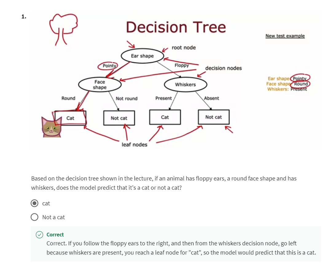
Correct. If you follow the floppy ears to the right, and then from the whiskers decision node, go left because whiskers are present, you reach a leaf node for “cat”, so the model would predict that this is a cat.

[3] Decision tree learning

Measuring purity

How to quantify how pure is the set of examples?

In this video, we’ll look
at the way of measuring the purity of a set of examples.

If the examples are all cats of a single class then
that’s very pure, if it’s all not cats
that’s also very pure, but if it’s somewhere
in between how do you quantify how pure is
the set of examples?

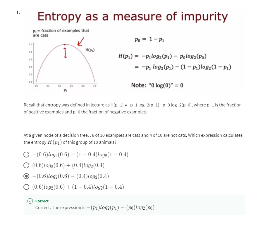
Entropy: a measure of the impurity of a set of data.

Let’s take a look at the
definition of entropy, which is a measure of the
impurity of a set of data.

$p_1$: the fraction of examples with label one

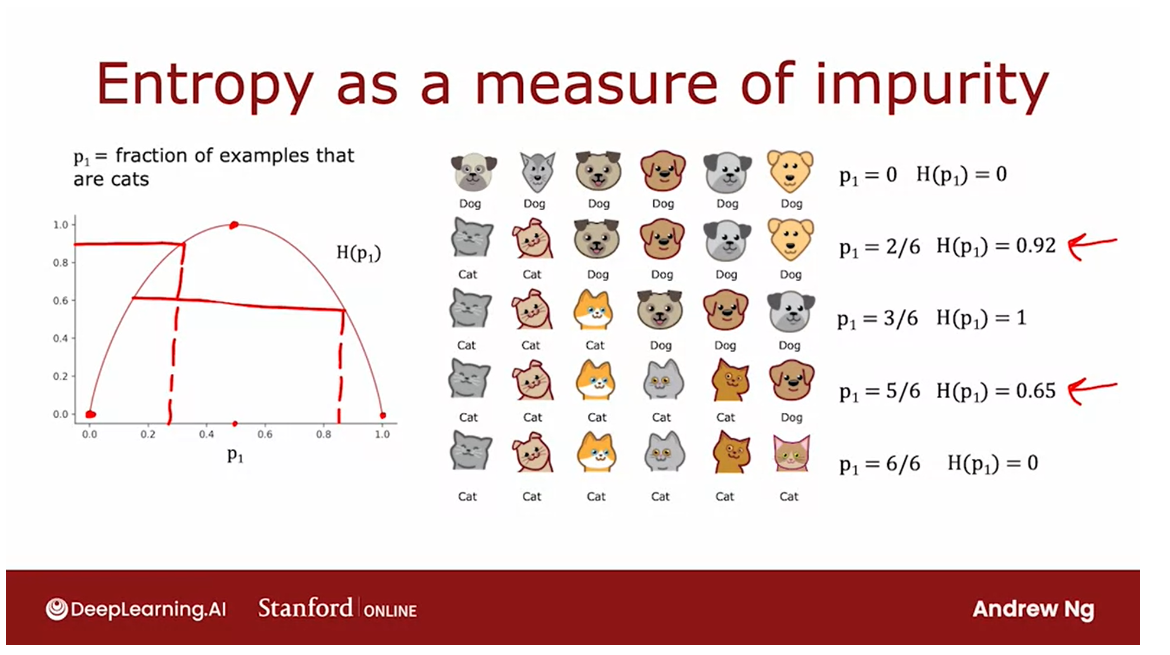
Given a set of six
examples like this, we have three cats
and three dogs, let’s define p_1 to be the fraction of
examples that are cats, that is, the fraction of
examples with label one, that’s what the
subscript one indicates.

p_1 in this example
is equal to 3/6. We’re going to measure the
impurity of a set of examples using a function called the entropy which
looks like this. The entropy function
is conventionally denoted as capital H of this number p_1 and the function looks
like this curve over here where the
horizontal axis is p_1, the fraction of
cats in the sample, and the vertical axis is
the value of the entropy.

In this example where
p_1 is 3/6 or 0.5, the value of the entropy of
p_1 would be equal to one.

You notice that this curve is highest when your set
of examples is 50-50, so it’s most impure as
an impurity of one or with an entropy of one when your set of
examples is 50-50, whereas in contrast if
your set of examples was either all cats or not cats
then the entropy is zero.

Let’s just go through a
few more examples to gain further intuition about
entropy and how it works.

Here’s a different
set of examples with five cats and one dog, so p_1 the fraction
of positive examples, a fraction of examples
labeled one is 5/6 and so p_1 is about 0.83. If you read off that value
at about 0.83 we find that the entropy of
p_1 is about 0.65.

Here I’m writing it only to two significant
digits and here I’m rounding it off to
two decimal points.

Here’s one more example. This sample of six images has all cats so p_1 is six out of six because all six are
cats and the entropy of p_1 is this point over
here which is zero.

We see that as you go from
3/6 to six out of six cats, the impurity decreases from one to zero or in other words, the purity increases as you go from a 50-50 mix of cats
and dogs to all cats.

Let’s look at a
few more examples. Here’s another sample with
two cats and four dogs, so p_1 here is 2/6 which is 1/3, and if you read
off the entropy at 0.33 it turns out
to be about 0.92.

This is actually quite
impure and in particular this set is more impure than this set because
it’s closer to a 50-50 mix, which is why the
impurity here is 0.92 as opposed to 0.65.

Finally, one last example, if we have a set of
all six dogs then p_1 is equal to 0 and
the entropy of p_1 is just this number down here
which is equal to 0 so there’s zero impurity or this would be a completely pure set of
all not cats or all dogs.

Don’t worry, we’ll
show the equation for the entropy of p_1
later in this video.

Now, let’s look at the
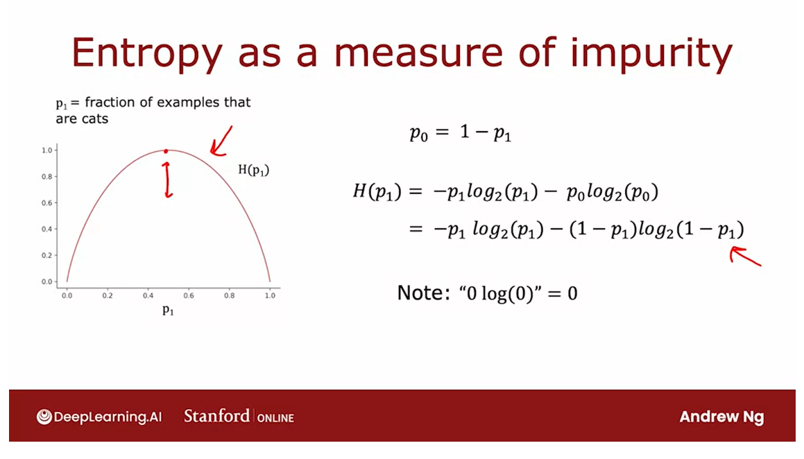
actual equation for the entropy function H(p_1).

Recall that p_1 is the fraction of examples that are equal to cats so if you
have a sample that is 2/3 cats then that sample
must have 1/3 not cats.

Let me define p_0 to be equal
to the fraction of examples that are not cats to be
just equal to 1 minus p_1. The entropy function
is then defined as negative p_1log_2 (p_1), and by convention when computing entropy we take logs to base two
rather than to base e, and then minus p_0log_2(p_0). Alternatively, this is also equal to negative p_1log_2(p_1) minus 1 minus p_1
log_2(1 minus p_1).

If you were to plot this function in a
computer you will find that it will be exactly
this function on the left.

We take log_2 just to make the peak of this
curve equal to one, if we were to take log_e or the base of natural logarithms, then that just vertically
scales this function, and it will still work but the numbers become a bit
hard to interpret because the peak of the function isn’t a nice round number
like one anymore.

One note on computing
this function, if p_1 or p_0 is equal to 0 then an expression like this
will look like 0log(0), and log(0) is
technically undefined, it’s actually negative infinity.

But by convention for the
purposes of computing entropy, we’ll take 0log(0) to be equal to 0 and that will correctly compute the entropy as zero or as one to be equal to zero.

If you’re thinking that this definition of entropy
looks a little bit like the definition of the logistic loss that we learned about in
the last course, there is actually a
mathematical rationale for why these two
formulas look so similar.

But you don’t have to
worry about it and we won’t get into it in this class. But applying this formula
for entropy should work just fine when you’re
building a decision tree.

To summarize, the
entropy function is a measure of the impurity
of a set of data. It starts from zero,
goes up to one, and then comes back down
to zero as a function of the fraction of positive
examples in your sample.

There are other functions
that look like this, they go from zero up to
one and then back down.

For example, if you look in
open source packages you may also hear about something
called the Gini criteria, which is another
function that looks a lot like the entropy function, and that will work well as well for building
decision trees.

But for the sake of simplicity, in these videos I’m
going to focus on using the entropy criteria which will usually work just fine
for most applications.

Now that we have this
definition of entropy, in the next video let’s take a look at how you can
actually use it to make decisions as to what
feature to split on in the nodes of
a decision tree.

Choosing a split: Information Gain

Reduce entropy (reduce impurity)

Choosing a split

What feature to split on at a node will be based on what choice of feature reduces entropy the most

When building a decision tree, the way we’ll decide what feature to split
on at a node will be based on what choice of feature
reduces entropy the most.

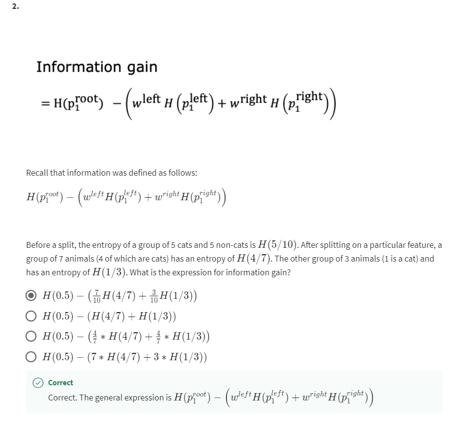
Information gain: reduction of entropy

Reduces entropy or reduces
impurity, or maximizes purity. In decision tree learning, the reduction of entropy is
called information gain.

Let’s take a look,
in this video, at how to compute information
gain and therefore choose what features to use to split on at each node
in a decision tree.

Let’s use the
example of deciding what feature to use
at the root node of the decision tree we
were building just now for recognizing cats
versus not cats.

Root node: use ear shape feature

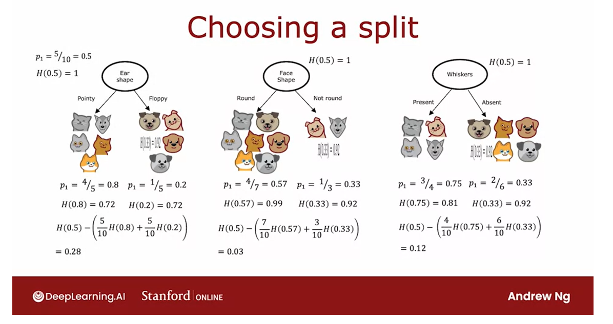
If we had split using their ear shape feature
at the root node, this is what we
would have gotten, five examples on the left
and five on the right.

On the left, we would have
four out of five cats, so P1 would be equal
to 4/5 or 0.8.

On the right, one out
of five are cats, so P1 is equal to 1/5 or 0.2.

If you apply the entropy
formula from the last video to this left subset of data and this
right subset of data, we find that the degree of impurity on the left
is entropy of 0.8, which is about 0.72, and on the right, the entropy of 0.2 turns
out also to be 0.72.

This would be the
entropy at the left and right subbranches if we were to split on the
ear shape feature.

Root node: use face shape feature

One other option would be to split on the face shape feature.

If we’d done so
then on the left, four of the seven
examples would be cats, so P1 is 4/7 and on the right, 1/3 are cats, so P1
on the right is 1/3.

The entropy of 4/7
and the entropy of 1/3 are 0.99 and 0.92. So the degree of
impurity in the left and right nodes
seems much higher, 0.99 and 0.92 compared
to 0.72 and 0.72.

Root node: use the whiskers feature

Finally, the third
possible choice of feature to use at the
root node would be the whiskers feature
in which case you split based on whether whiskers are present or absent.

In this case, P1 on
the left is 3/4, P1 on the right is 2/6, and the entropy values
are as follows.

Which one do we think works best?

The key question we
need to answer is, given these three options of a feature to use
at the root node, which one do we
think works best?

It turns out that
rather than looking at these entropy numbers
and comparing them, it would be useful to take a weighted average of them,
and here’s what I mean.

If there’s a node with a lot of examples in it with high entropy that seems worse than
if there was a node with just a few examples
in it with high entropy.

Because entropy, as a
measure of impurity, is worse if you have a very large and impure
dataset compared to just a few examples and a branch of the tree
that is very impure.

The key decision is, of these three possible choices of features to use
at the root node, which one do we want to use?

Associated with each of
these splits is two numbers, the entropy on the
left sub-branch and the entropy on
the right sub-branch.

Combine the subbranch numbers into a single number

In order to pick from these, we like to actually combine these two numbers
into a single number. So you can just pick of these three choices,
which one does best?

The way we’re going to combine these two numbers is by
taking a weighted average.

Because how important it is to have low entropy in, say, the left or right
sub-branch also depends on how many examples went into
the left or right sub-branch.

Because if there are lots
of examples in, say, the left sub-branch
then it seems more important to make sure that that left sub-branch’s
entropy value is low.

In this example we have, five of the 10 examples went
to the left sub-branch, so we can compute
the weighted average as 5/10 times the
entropy of 0.8, and then add to
that 5/10 examples also went to the
right sub-branch, plus 5/10 times the
entropy of 0.2.

Now, for this example
in the middle, the left sub-branch had received seven out
of 10 examples. and so we’re going to compute 7/10 times the
entropy of 0.57 plus, the right sub-branch had
three out of 10 examples, so plus 3/10 times
entropy of 0.3 of 1/3.

Finally, on the right, we’ll compute 4/10
times entropy of 0.75 plus 6/10 times
entropy of 0.33.

The way we will
choose a split is by computing these three numbers
and picking whichever one is lowest because that
gives us the left and right sub-branches with the lowest average
weighted entropy.

In the way that decision
trees are built, we’re actually going to
make one more change to these formulas to stick to the convention in
decision tree building, but it won’t actually
change the outcome.

Compute the reduction in entropy

Entropy - weighted average entropy

Which is rather than computing this weighted average entropy, we’re going to compute
the reduction in entropy compared to if
we hadn’t split at all.

If we go to the root node, remember that the root node
we have started off with all 10 examples in the root node with five cats and dogs, and so at the root node, we had p_1 equals 5/10 or 0.5.

The entropy of the root nodes, entropy of 0.5 was
actually equal to 1.

This was maximum in purity because it was five
cats and five dogs.

The formula that we’re
actually going to use for choosing a split is not this way to entropy at the left and right sub-branches, instead is going to be the
entropy at the root node, which is entropy of 0.5, then minus this formula.

In this example, if
you work out the math, it turns out to be 0.28.

For the face shape example, we can compute entropy
of the root node, entropy of 0.5 minus this, which turns out to be
0.03, and for whiskers, compute that, which
turns out to be 0.12.

Information gain 这些被称为信息增益，它衡量的是由于进行拆分而在树中得到的熵的减少。

These numbers that
we just calculated, 0.28, 0.03, and 0.12, these are called the
information gain, and what it measures
is the reduction in entropy that you get in your tree resulting
from making a split.

Because the entropy
was originally one at the root node and
by making the split, you end up with a lower
value of entropy and the difference between
those two values is a reduction in entropy, and that’s 0.28 in the case of splitting
on the ear shape.

为什么要比较熵的减少呢？

Why do we bother to
compute reduction in entropy rather than just entropy at the left and
right sub-branches?

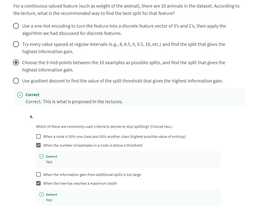
one of the stopping criteria for deciding when to not bother to split any further is if the reduction in entropy is too small.

结果表明，决定何时不再进行进一步拆分的停止标准之一是熵的减少是否太小。

在这种情况下，你可以决定，你只是不必要地增加了树的大小，并冒着通过拆分过度拟合的风险，只是决定如果熵的减少太小或低于阈值，就不要麻烦了。

It turns out that one of the stopping criteria
for deciding when to not bother to split any further is if the reduction in
entropy is too small.

In which case you could decide, you’re just increasing
the size of the tree unnecessarily and
risking overfitting by splitting and just
decide to not bother if the reduction in entropy is too small or
below a threshold.

In this other example, spitting on ear shape results in the biggest
reduction in entropy, 0.28 is bigger than 0.03 or 0.12 and so we would
choose to split onto ear shape feature
at the root node.

On the next slide, let’s give a more formal definition
of information gain.

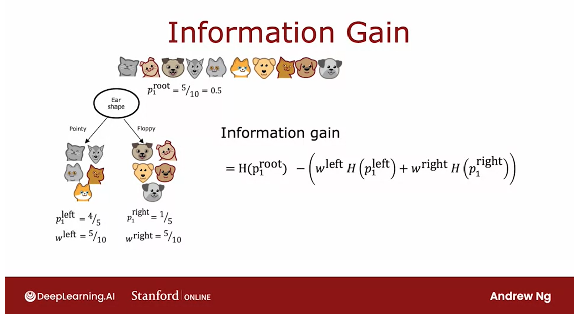
$w^{left}$: the fraction of examples that went to the left branch

$w^{right}$: the fraction of examples that went to the right branch

By the way, one additional piece of notation that we’ll introduce also in the next slide is
these numbers, 5/10 and 5/10.

I’m going to call
this w^left because that’s the fraction of examples that went
to the left branch, and I’m going to
call this w^right because that’s the fraction of examples that went
to the right branch.

Whereas for this
another example, w^left would be 7/10, and w^right will be 3/10.

Let’s now write down the general formula for how
to compute information gain.

Using the example of splitting
on the ear shape feature, let me define p_1^left
to be equal to the fraction of examples in the left subtree that have a positive label, that are cats.

In this example, p_1^left
will be equal to 4/5.

Also, let me define w^left
to be the fraction of examples of all of
the examples of the root node that went
to the left sub-branch, and so in this example,
w^left would be 5/10.

Similarly, let’s define p_1^right to be of all the
examples in the right branch. The fraction that are
positive examples and so one of the five of
these examples being cats, there’ll be 1/5, and similarly, w^right is 5/10 the fraction of examples that went to
the right sub-branch.

$p_1^{root}$ to be the fraction of examples that are positive in the root node.

Let’s also define p_1^root to be the fraction of examples that are positive in the root node. In this case, this
would be 5/10 or 0.5.

Information gain = entropy of root node - weighted average entropy

Information gain
is then defined as the entropy of p_1^root, so what’s the entropy
at the root node, minus that weighted
entropy calculation that we had on the
previous slide, minus w^left those were
5/10 in the example, times the entropy
applied to p_1^left, that’s entropy on
the left sub-branch, plus w^right the fraction of examples that went
to the right branch, times entropy of p_1^right.

With this definition of entropy, and you can calculate the
information gain associated with choosing any
particular feature to split on in the node.

out of all the possible futures, you could choose to split on, you can then pick the one that gives you the highest information gain.

Then out of all the
possible futures, you could choose to split on, you can then pick the
one that gives you the highest information gain.

That will result in, hopefully, increasing the purity
of your subsets of data that you get on the
left and right sub-branches of your decision tree and that will result in choosing
a feature to split on that increases the purity of your subsets of data in both the left and right sub-branches of
your decision tree.

Now that you know
how to calculate information gain or
reduction in entropy, you know how to pick a feature
to split on another node. Let’s put all the things we’ve
talked about together into the overall algorithm for building a decision tree
given a training set. Let’s go see that
in the next video.

Putting it together

The information gain
criteria lets you decide how to choose one feature
to split a one-node.

Let’s take that and use that
in multiple places through a decision tree in order
to figure out how to build a large decision
tree with multiple nodes.

Here is the overall process
of building a decision tree.

Pick the feature that gives the highest information gain

Starts with all
training examples at the root node of the tree and calculate the
information gain for all possible features and
pick the feature to split on, that gives the highest
information gain.

Having chosen this feature, you would then split
the dataset into two subsets according to
the selected feature, and create left and right
branches of the tree and send the training examples to either the left
or the right branch, depending on the value of that
feature for that example.

Keep on repeating the splitting process

This allows you to have made
a split at the root node.

After that, you will
then keep on repeating the splitting process on the
left branch of the tree, on the right branch of
the tree and so on.

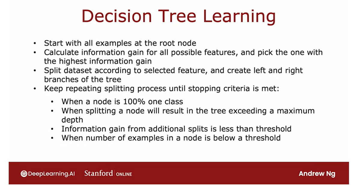
Keep on doing that until the
stopping criteria is met.

Where the stopping
criteria can be, when a node is 100
percent a single clause, someone has reached
entropy of zero, or when further splitting
a node will cause the tree to exceed the maximum
depth that you had set, or if the information gain from an additional splits is
less than the threshold, or if the number of examples in a nodes
is below a threshold.

You will keep on repeating
the splitting process until the stopping criteria
that you’ve chosen, which could be one or more
of these criteria is met.

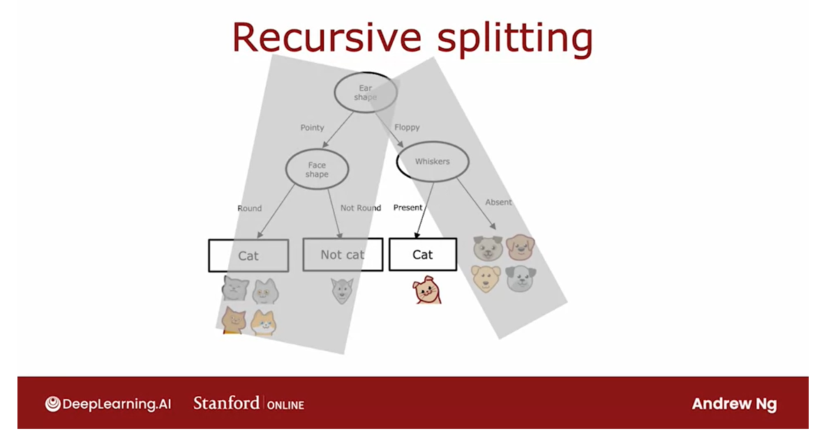
Let’s look at an illustration of how this process will work.

We started all of
the examples at the root nodes and based on computing information gain
for all three features, decide that ear-shaped is the
best feature to split on.

Based on that, we create a left and right sub-branches and send the subsets of the data
with pointy versus floppy ear to left and
right sub-branches.

Let me cover the root node and the right sub-branch
and just focus on the left sub-branch where we
have these five examples.

Let’s see off splitting
criteria is to keep splitting until everything in the node
belongs to a single class, so either all cancel all nodes.

We will look at this node and see if it meets the
splitting criteria, and it does not because there is a mix of cats and dogs here.

The next step is to then
pick a feature to split on.

We then go through the features
one at a time and compute the information gain of each of those features as if this node, were the new root node of
a decision tree that was trained using just five
training examples shown here.

We would compute the
information gain for splitting on the
whiskers feature, the information gain on splitting
on the V-shape feature.

It turns out that
the information gain for splitting on
ear shape will be zero because all of these have
the same point ear shape.

Between whiskers and V-shape, V-shape turns out to have a
highest information gain. We’re going to split
on V-shape and that allows us to build left and right sub
branches as follows.

Then for the left
sub-branch here, we check for the
stopping criteria and we find that is all cats.

We stop splitting and build a prediction node
that predicts cat, and for the right sub-branch, we again check the
stopping criteria and we find that is all dogs.

We stop splitting and
have a prediction node.

For the left sub-branch, we check for the criteria
for whether or not we should stop splitting
and we have all cats here.

The stopping criteria
is met and we create a leaf node that makes
a prediction of cat.

For the right sub-branch, we find that it is all dogs. We will also stop
splitting since we’ve met the splitting criteria and
put a leaf node there, that predicts not cat.

Having built out
this left subtree, we can now turn our attention to building the right subtree.

Let me now again cover up the root node and the
entire left subtree.

To build out the right subtree, we have these five
examples here.

Again, the first thing
we do is check if the criteria to stop
splitting has been met, their criteria being met or not.

All the examples are
a single clause, we’ve not met that criteria.

We’ll decide to keep splitting in this right
sub-branch as well.

In fact, the procedure
for building the right sub-branch
will be a lot as if you were training a decision tree learning
algorithm from scratch, where the dataset you have comprises just these
five training examples.

Again, computing
information gain for all of the possible
features to split on, you find that the
whiskers feature use the highest
information gain.

Split this set of five examples according to whether whiskers
are present or absent.

Check if the criteria to
stop splitting are met in the left and right sub-branches here and
decide that they are.

You end up with leaf nodes
that predict cat and dog cat.

This is the overall process for building the decision tree.

Notice that there’s interesting aspects
of what we’ve done, which is after we
decided what to split on at the root node, the way we built the
left subtree was by building a decision tree on
a subset of five examples.

The way we built the right
subtree was by, again, building a decision tree on
a subset of five examples.

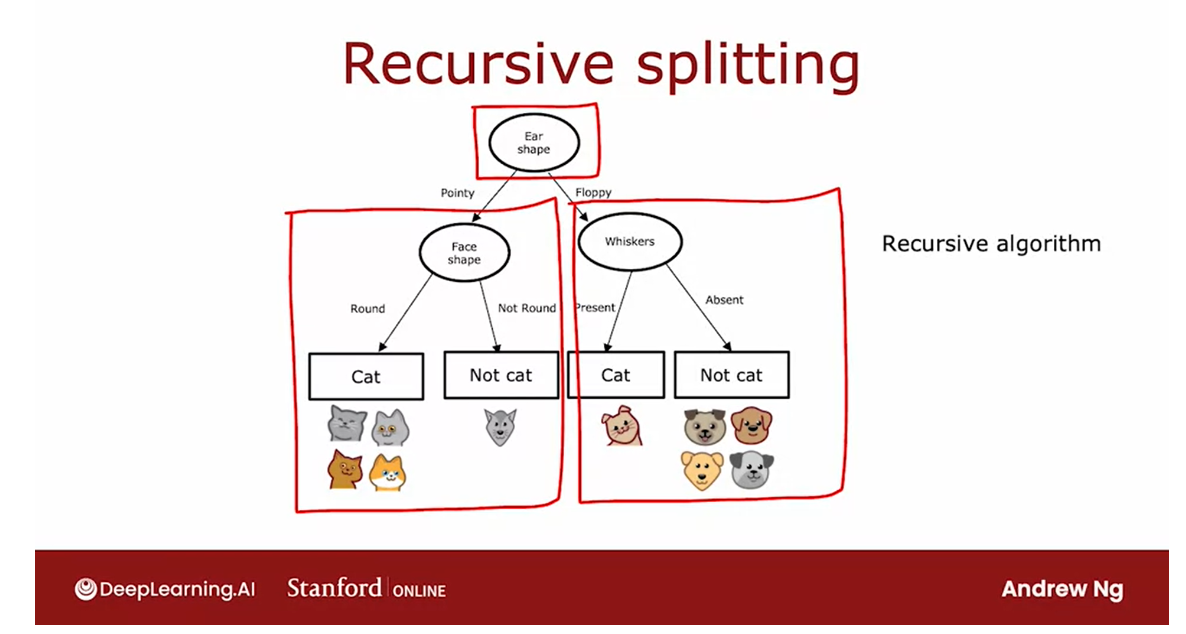
In computer science,
this is an example of a recursive algorithm.

All that means is
the way you build a decision tree
at the root is by building other smaller
decision trees in the left and the
right sub-branches.

Recursion in computer science refers to writing code
that calls itself.

The way this comes up in
building a decision tree is you build the overall
decision tree by building smaller sub-decision trees and then putting them all together.

That’s why if you look at software implementations
of decision trees, you’ll see sometimes references
to a recursive algorithm.

But if you don’t feel like
you’ve fully understood this concept of
recursive algorithms, don’t worry about it.

You still be able to fully complete this
week’s assignments, as well as use libraries to get decision trees to
work for yourself.

But if you’re implementing a decision tree
algorithm from scratch, then a recursive algorithm turns out to be one of the steps
you’d have to implement.

By the way, you may
be wondering how to choose the maximum
depth parameter.

There are many different
possible choices, but some of the
open-source libraries will have good default choices
that you can use.

One intuition is, the
larger the maximum depth, the bigger the decision tree
you’re willing to build.

This is a bit like fitting a higher degree polynomial or training a larger
neural network.

It lets the decision tree
learn a more complex model, but it also increases
the risk of overfitting if this fitting a very complex
function to your data.

In theory, you could use cross-validation
to pick parameters like the maximum depth, where you try out
different values of the maximum depth and pick what works best on
the cross-validation set.

Although in practice, the
open-source libraries have even somewhat better ways to choose this
parameter for you.

Or another criteria that you can use to decide
when to stop splitting is if the information gained from an additional slit is
less than a certain threshold.

If any feature is splint on, achieves only a small
reduction in entropy or a very small
information gain, then you might also
decide to not bother.

Finally, you can also
decide to start splitting when the number of examples in the node is below a
certain threshold.

That’s the process of
building a decision tree.

Now that you’ve learned
the decision tree, if you want to
make a prediction, you can then follow
the procedure that you saw in the very first
video of this week, where you take a new example, say a test example, and started a route and keep on following the decisions down
until you get to leaf note, which then makes the prediction.

Now that you know the basic decision tree
learning algorithm, in the next few videos, I’d like to go into some further refinements
of this algorithm.

So far we’ve only used features to take on two possible values. But sometimes you have a feature that takes on
categorical or discrete values, but maybe more than two values. Let’s take a look in
the next video at how to handle that case.

Using one-hot encoding of categorical features

In the example we’ve seen so far each of the features could take
on only one of two possible values.

The ear shape was either pointy or floppy,
the face shape was either round or not round and
whiskers were either present or absent.

Have features that can take on more than two discrete values

But whether if you have features that can
take on more than two discrete values, in this video we’ll look at how
you can use one-hot encoding to address features like that.

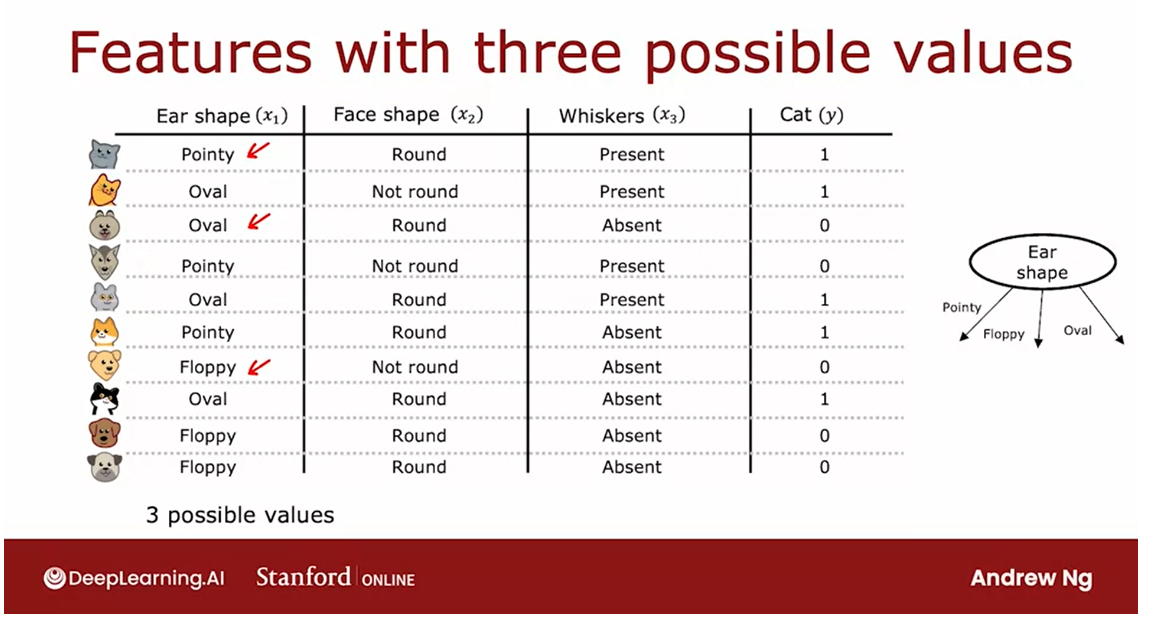
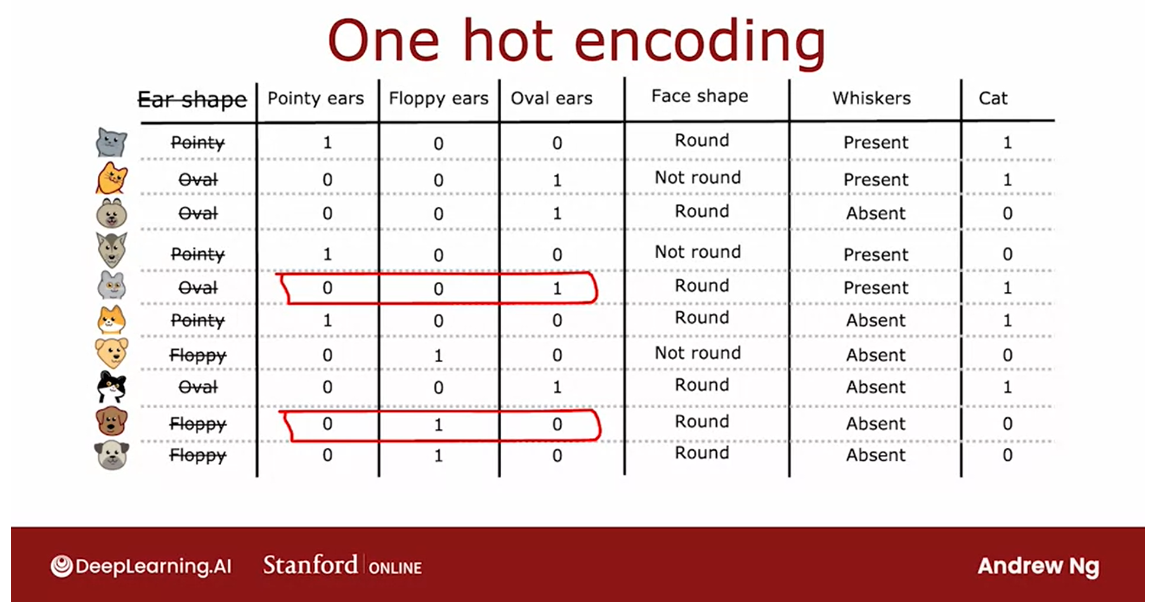
Here’s a new training set for
our pet adoption center application where all the data is the same except for
the ear shaped feature.

Rather than ear shape only
being pointy and floppy, it can now also take on an oval shape.

And so the initial feature is still
a categorical value feature but it can take on three possible values
instead of just two possible values.

And this means that when you split
on this feature you end up creating three subsets of the data and end up
building three sub branches for this tree.

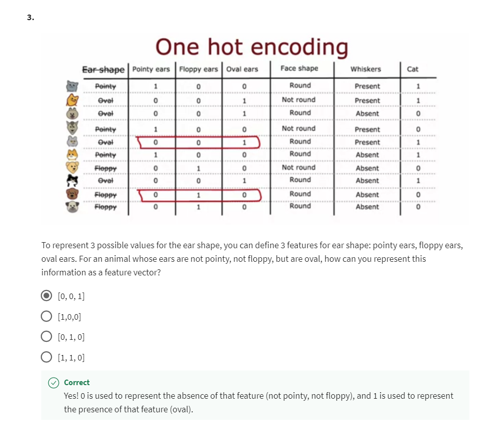
But in this video I’d like to describe
a different way of addressing features that can take on more than two values,
which is to use the one-hot encoding.

In particular rather than
using an ear shaped feature, they can take on any of
three possible values. We’re instead going to create three
new features where one feature is, does this animal have pointy ears,
a second is does their floppy ears and the third is does it have oval ears.

And so for the first example whereas
we previously had ear shape as pointy, we are now instead say that
this animal has a value for the pointy ear feature of 1 and
0 for floppy and oval.

Whereas previously for the second example, we previously said it had oval ears now
we’ll say that it has a value of 0 for pointy ears because it
doesn’t have pointy ears.

It also doesn’t have floppy ears but
it does have oval ears which is why this value here is 1 and so on for
the rest of the examples in the data set.

And so instead of one feature
taking on three possible values, we’ve now constructed three new
features each of which can take on only one of two possible values,
either 0 or 1.

In a little bit more detail,
if a categorical feature can take on k possible values, k was three in
our example, then we will replace it by creating k binary features that
can only take on the values 0 or 1.

And you notice that among
all of these three features, if you look at any role here,
exactly 1 of the values is equal to 1.

And that’s what gives this method of
future construction the name one-hot encoding.

And because one of these features will
always take on the value 1 that’s the hot feature and
hence the name one-hot encoding.

And with this choice of features we’re
now back to the original setting of where each feature only takes on one
of two possible values, and so the decision tree learning algorithm
that we’ve seen previously will apply to this data with no further modifications.

the idea of using one-hot encodings to encode categorical features also works for training neural networks.

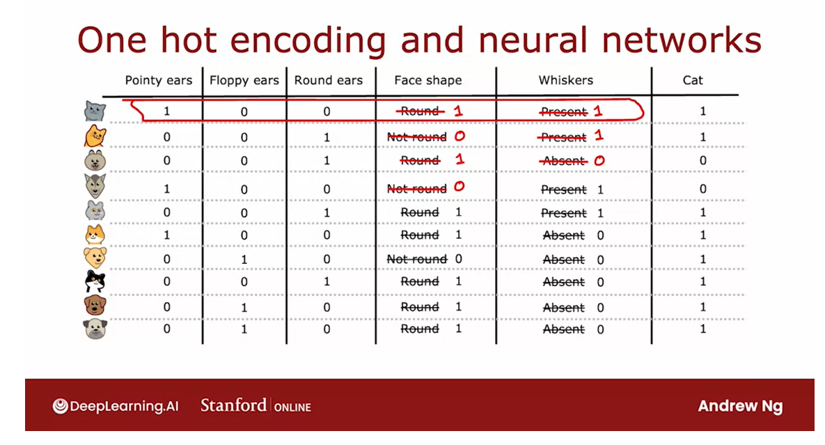
Just in the side, even though this
week’s material has been focused on training decision tree models the idea
of using one-hot encodings to encode categorical features also works for
training neural networks.

In particular if you were to
take the face shape feature and replace round and not round with 1 and 0 where round gets matter 1,
not round gets matter 0 and so on.

And for whiskers similarly replace
presence with 1 and absence with 0.

They noticed that we have taken all
the categorical features we had where we had three possible values for
ear shape, two for face shape and one for whiskers and
encoded as a list of these five features.

Three from the one-hot encoding of
ear shape, one from face shape and from whiskers and now this list of
five features can also be fed to a new network or to logistic regression
to try to train a cat classifier.

encode categorical features using ones and zeros, so that it can be fed as inputs to a neural network as well which expects numbers as inputs.

So one-hot encoding is a technique that
works not just for decision tree learning but also lets you encode categorical
features using ones and zeros, so that it can be fed as inputs to a neural network
as well which expects numbers as inputs.

So that’s it, with a one-hot encoding you
can get your decision tree to work on features that can take on more than two
discrete values and you can also apply this to new network or linear regression
or logistic regression training.

But how about features that are numbers
that can take on any value, not just a small number
of discrete values. In the next video let’s look at how you
can get the decision tree to handle continuous value features
that can be any number.

Continuous valued features

Features that can be any number

Let’s look at how you can modify
decision tree to work with features that aren’t just discrete
value but continuous value.

That is features that can be any number.

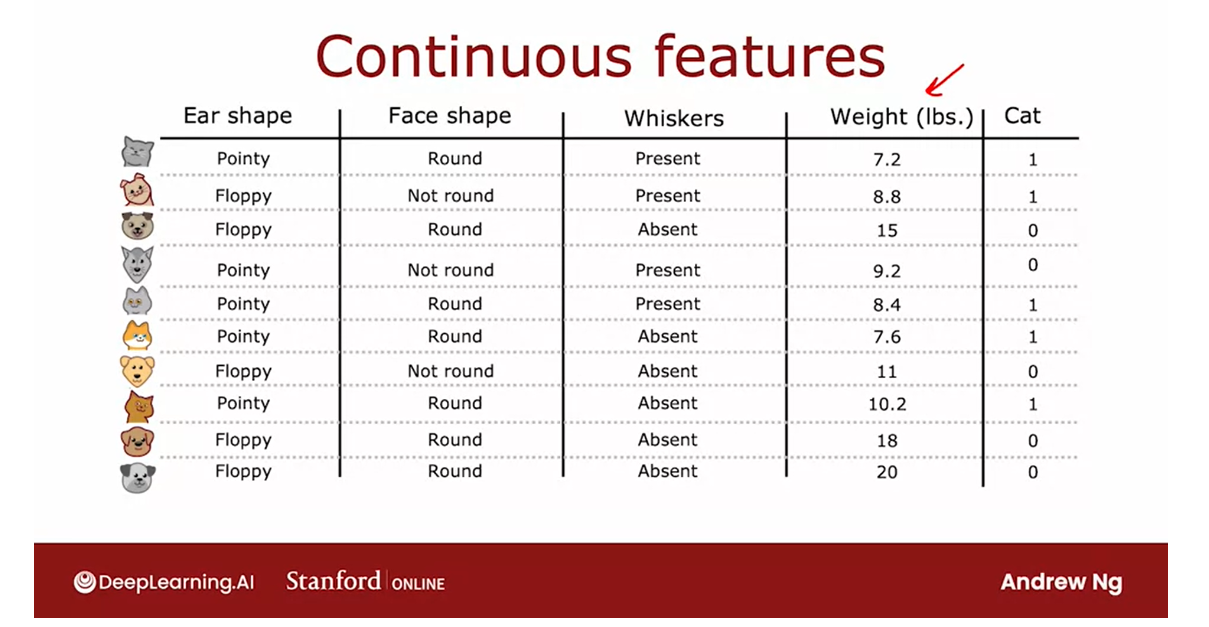
Let’s start with an example,
I have modified the cat adoption center of data set to add one more feature
which is the weight of the animal.

In pounds on average between cats and
dogs, cats are a little bit lighter than dogs, although there are some
cats are heavier than some dogs.

But so the weight of an animal
is a useful feature for deciding if it is a cat or not.

So how do you get a decision
tree to use a feature like this? The decision tree learning algorithm will
proceed similarly as before except that rather than constraint splitting just
on ear shape, face shape and whiskers.

You have to consist splitting on ear
shape, face shape whisker or weight. And if splitting on the weight
feature gives better information gain than the other options.

Then you will split on the weight feature.

But how do you decide how to
split on the weight feature? Let’s take a look.

Here’s a plot of the data at the root. Not a plotted on the horizontal axis.

The way to the animal and the vertical
axis is cat on top and not cat below. So the vertical axis indicates the label,
y being 1 or 0.

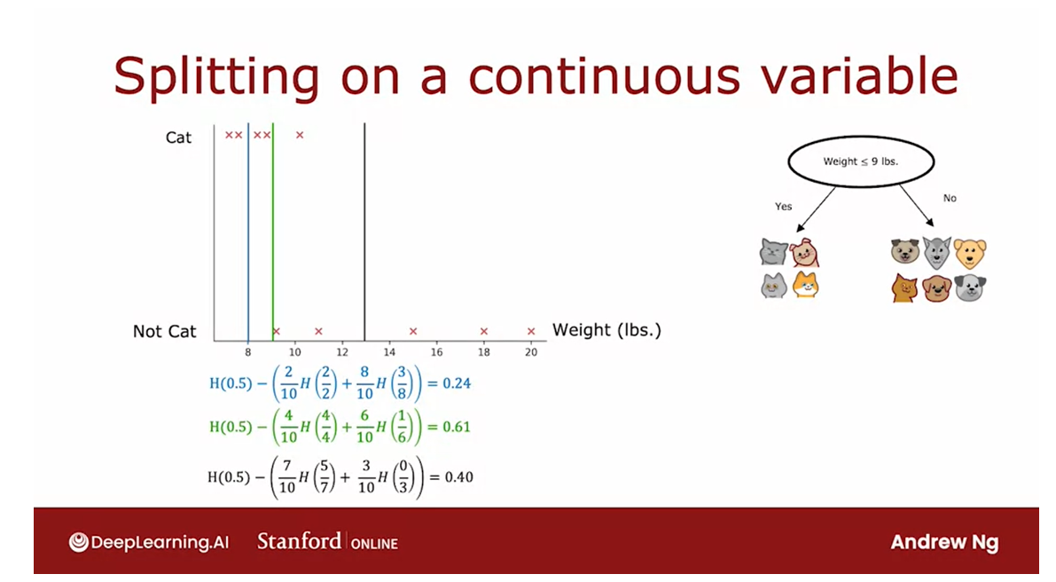
The way we were split on the weight
feature would be if we were to split the data based on whether or
not the weight is less than or equal to some value.

Let’s say 8 or some of the number.

That will be the job of
the learning algorithm to choose.

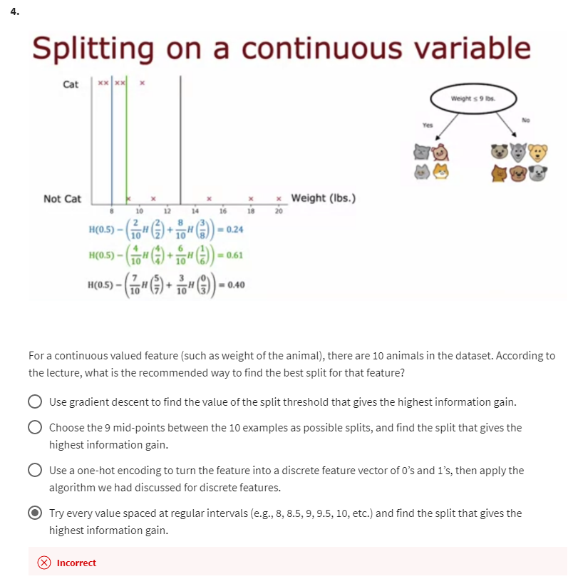
When constraints splitting on the weight feature, consider many different values of the threshold and then to pick the one that is the best (resulting in the best information gain).

And what we should do when
constraints splitting on the weight feature is to consider many different
values of this threshold and then to pick the one that is the best.

And by the best I mean the one that
results in the best information gain.

So in particular, if you were
considering splitting the examples based on whether the weight
is less than or equal to 8, then you will be splitting this
data set into two subsets.

Where the subset on
the left has two cats and the subset on the right has three cats and
five dogs.

So if you were to calculate our
usual information gain calculation, you’ll be computing the entropy
at the root note N C p f 0.5 minus now 2/10 times entropy of
the left split has two other two cats. So it should be 2/2 plus
the right split has eight out of 10 examples and an entropy F.

That’s of the eight examples
on the right three cats. To entry of 3/8 and
this turns out to be 0.24.

So this would be information gain if you
were to split on whether the weight is less than equal to 8 but
we should try other values as well.

So what if you were to split on whether or
not the weight is less than equal to 9 and that corresponds to this
new line over here. And the information gain
calculation becomes H (0.5) minus.

So now we have four examples and
left split all cats. So that’s 4/10 times
entropy of 4/4 plus six examples on the right of
which you have one cat.

So that’s 6/10 times each of 1/6,
which is equal to turns out 0.61. So the information gain here
looks much better is 0.61 information gain which is
much higher than 0.24.

Or we could try another value say 13. And the calculation turns out to
look like this, which is 0.40.

And one convention would be to sort all of the examples according to the weight or according to the value of this feature and take all the values that are mid points between the sorted list of training.

In the more general case,
we’ll actually try not just three values, but multiple values along the X axis. And one convention would be to sort all of
the examples according to the weight or according to the value of this feature and take all the values that are mid points
between the sorted list of training.

Examples as the values for consideration
for this threshold over here.

This way,
if you have 10 training examples, you will test nine different possible
values for this threshold and then try to pick the one that gives
you the highest information gain.

And finally, if the information gained
from splitting on a given value of this threshold is better than the information
gain from splitting on any other feature, then you will decide to split
that note at that feature.

And in this example an information
gain of 0.61 turns out to be higher than that of any other feature.

It turns out they’re
actually two thresholds.

And so assuming the algorithm
chooses this feature to split on, you will end up splitting the data
set according to whether or not the weight of the animal
is less than equal to £9.

And so you end up with two
subsets of the data like this and you can then build recursive,
li additional decision trees using these two subsets of the data to
build out the rest of the tree.

When consuming splits, you would just consider different values to split on, carry out the usual information gain calculation and decide to split on that continuous value feature if it gives the highest possible information gain.

So to summarize to get
the decision tree to work on continuous value
features at every note.

When consuming splits, you would just
consider different values to split on, carry out the usual information gain
calculation and decide to split on that continuous value feature if it gives
the highest possible information gain.

So that’s how you get the decision tree
to work with continuous value features.

Try different thresholds, do the usual
information gain calculation and split on the continuous value feature with
the selected threshold if it gives you the best possible information gain out
of all possible features to split on.

And that’s it for the required videos
on the core decision tree algorithm.

After there’s there is an optional
video you can watch or not that generalizes the decision tree
learning algorithm to regression trees.

So far, we’ve only talked about using
decision trees to make predictions that are classifications predicting a discrete
category, such as cat or not cat. But what if you have a regression
problem where you want to predict a number in the next video. I’ll talk about a generalization
of decision trees to handle that.

Regression Trees (optional)

回归树（可选）

So far we’ve only been talking about
decision trees as classification algorithms.

Generalize decision trees to be regression algorithms so that we can predict a number.

In this optional video, we’ll generalize
decision trees to be regression algorithms so
that we can predict a number.

Let’s take a look.

The example I’m going to use for this video will be to use the this
three features that we had previously, that is, these features X, In order to
predict the weight of the animal, Y.

So just to be clear, the weight here, unlike the previous video is
no longer an input feature.

Instead, this is the target output,
Y, that we want to predict rather than trying to predict whether or
not an animal is or is not a cat.

This is a regression problem because
we want to predict a number, Y.

Let’s look at what a regression
tree will look like.

Here I’ve already constructed a tree for
this regression problem where the root node splits on
ear shape and then the left and right sub tree split on face shape and
also face shape here on the right.

And there’s nothing wrong with
a decision tree that chooses to split on the same feature in both the left and
right side branches.

It’s perfectly fine if the splitting
algorithm chooses to do that.

If during training,
you had decided on these splits, then this node down here would
have these four animals with weights 7.2, 7.6 and 10.2.

This node would have this one
animal with weight 9.2 and so on for these remaining two nodes.

So, the last thing we need to fill in for
this decision tree is if there’s a test example that comes down to
this node, what is there weights that we should predict for an animal with
pointy ears and a round face shape?

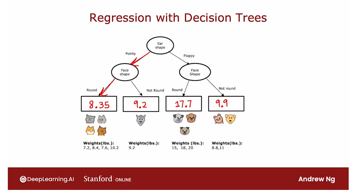
Make a prediction: take the average of the weights

The decision tree is going to
make a prediction based on taking the average of the weights in
the training examples down here.

And by averaging these four numbers,
it turns out you get 8.35.

If on the other hand,
an animal has pointy ears and a not round face shape,
then it will predict 9.2 or 9.2 pounds because that’s the weight
of this one animal down here.

And similarly,
this will be 17.70 and 9.90.

So, what this model will do is given
a new test example, follow the decision nodes down as usual until it gets to
a leaf node and then predict that value at the leaf node which I had just computed
by taking an average of the weights of the animals that during training had
gotten down to that same leaf node.

So, if you were constructing a decision
tree from scratch using this data set in order to predict the weight.

The key decision as you’ve seen
earlier this week will be, how do you choose which
feature to split on?

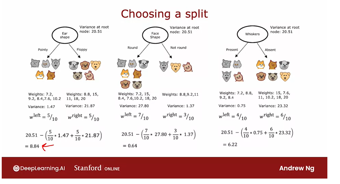
Let me illustrate how to make
that decision with an example.

At the root node, one thing you could
do is split on the ear shape and if you do that, you end up with left and
right branches of the tree with five animals on the left and
right with the following weights.

If you were to choose the spit on the face
shape, you end up with these animals on the left and right with the corresponding
weights that are written below.

And if you were to choose to split
on whiskers being present or absent, you end up with this.

So, the question is,
given these three possible features to split on at the root node,
which one do you want to pick that gives the best predictions for
the weight of the animal?

Build a regression tree: reduce the variance of the weight of the values Y at each of these subsets of the data.

When building a regression tree,
rather than trying to reduce entropy, which was that measure of
impurity that we had for a classification problem,
we instead try to reduce the variance of the weight of the values Y at
each of these subsets of the data.

So, if you’ve seen the notion of variants
in other contexts, that’s great.

This is the statistical mathematical
notion of variants that we’ll used in a minute.

But if you’ve not seen how to compute
the variance of a set of numbers before, don’t worry about it.

Variance: compute how widely a set of numbers varies

All you need to know for
this slide is that variants informally computes how widely
a set of numbers varies.

So for this set of numbers 7.2,
9.2 and so on, up to 10.2, it turns out the variance is 1.47,
so it doesn’t vary that much.

Whereas, here 8.8, 15, 11, 18 and 20, these numbers go all the way
from 8.8 all the way up to 20.

And so the variance is much larger,
turns out to the variance of 21.87.

And so the way we’ll evaluate
the quality of the split is, we’ll compute same as before, W left and W right as the fraction of examples that
went to the left and right branches.

And the average variance after
the split is going to be 5/10, which is W left times 1.47,
which is the variance on the left and then plus 5/10 times the variance
on the right, which is 21.87.

Weighted average variance

So, this weighted average variance plays
a very similar role to the weighted average entropy that we had used
when deciding what split to use for a classification problem.

And we can then repeat
this calculation for the other possible choices
of features to split on.

Here in the tree in the middle, the variance of these numbers
here turns out to be 27.80. The variance here is 1.37.

And so with W left equals seven-tenths and
W right as three-tenths, and so with these values, you can compute
the weighted variance as follows.

Finally, for the last example, if you
were to split on the whiskers feature, this is the variance on the left and
right, there’s W left and W right.

And so the weight of variance is this.

A good way to choose a split would be to just choose the value of the weighted variance that is lowest.

A good way to choose a split would
be to just choose the value of the weighted variance that is lowest.

Similar to when we’re
computing information gain, I’m going to make just one more
modification to this equation.

Just as for the classification problem, we
didn’t just measure the average weighted entropy, we measured the reduction in
entropy and that was information gain.

Measure the reduction in variance.

For a regression tree we’ll also similarly
measure the reduction in variance.

Turns out, if you look at all of
the examples in the training set, all ten examples and
compute the variance of all of them, the variance of all the examples
turns out to be 20.51.

And that’s the same value for
the roots node in all of these, of course, because it’s the same
ten examples at the roots node.

And so what we’ll actually compute
is the variance of the roots node, which is 20.51 minus this expression down
here, which turns out to be equal to 8.84.

And so at the roots node, the variance was
20.51 and after splitting on ear shape, the average weighted variance at
these two nodes is 8.84 lower.

So, the reduction in variance is 8.84.

And similarly, if you compute the
expression for reduction in variance for this example in the middle, it’s 20.51
minus this expression that we had before, which turns out to be equal to 0.64. So, this is a very small
reduction in variance.

And for the whiskers feature you
end up with this which is 6.22.

So, between all three of these examples, 8.84 gives you the largest
reduction in variance.

evaluating different options of features to split on and picking the one that gives you the biggest variance reduction.

So, just as previously we would
choose the feature that gives you the largest information gain for
a regression tree, you will choose the feature that gives
you the largest reduction in variance, which is why you choose ear shape
as the feature to split on.

Having chosen the year shaped features
to spit on, you now have two subsets of five examples in the left and
right side branches and you would then, again, we say recursively,
where you take these five examples and do a new decision tree focusing
on just these five examples, again, evaluating different options
of features to split on and picking the one that gives you
the biggest variance reduction.

And similarly on the right.

And you keep on splitting until
you meet the criteria for not splitting any further. And so that’s it.

With this technique, you can get your
decision treat to not just carry out classification problems,
but also regression problems.

So far, we’ve talked about how
to train a single decision tree.

An ensemble of decision trees

It turns out if you train
a lot of decision trees, we call this an ensemble of decision
trees, you can get a much better result.

Let’s take a look at why and
how to do so in the next video.

[4] Practice quiz: Decision tree learning

Practice quiz: Decision tree learning

Latest Submission Grade 80% 这是第一次尝试

Practice quiz: Decision tree learning

Latest Submission Grade 100% 这是第二次尝试

Question 4 correct answer

[5] Tree ensembles

Using multiple decision trees

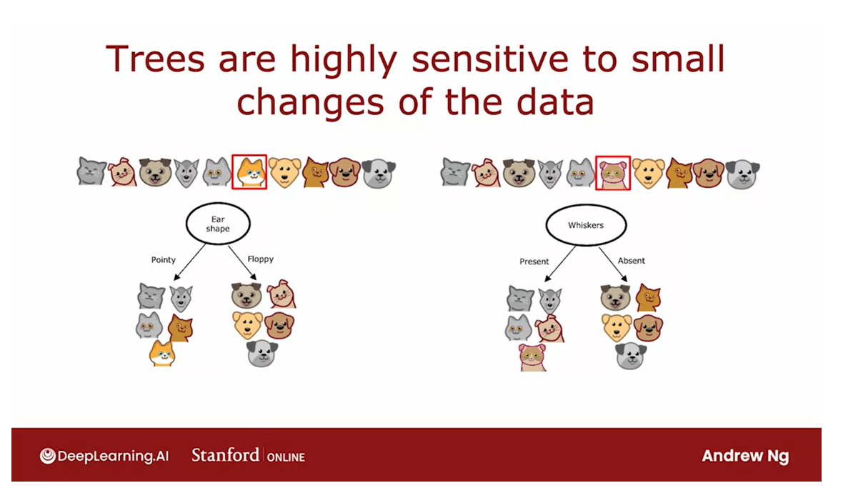
A single decision tree: can be highly sensitive to small changes in the data

Solution: build a lot of decision trees, and we call that a tree ensemble

One of the weaknesses of using a single decision tree is that that decision tree can be highly sensitive to small
changes in the data.

One solution to make the
arrow less sensitive or more robust is to build
not one decision tree, but to build a lot
of decision trees, and we call that
a tree ensemble.

Let’s take a look.
With the example that we’ve been using, the best feature to split
on at the root node turned out to be the
ear shape resulting in these two subsets of
the data and then building further sub trees on these two subsets of the data.

But it turns out
that if you were to take just one of the
ten examples and change it to a different cat so that instead of
having pointy ears, round face, whiskers absent, this new cat has floppy ears, round face, whiskers present, with just changing a
single training example, the highest information
gain feature to split on becomes the whiskers feature instead of the ear
shape feature.

As a result of that, the subsets of data you get in the left and right
sub-trees become totally different and as you continue to run the decision tree learning
algorithm recursively, you build out totally
different sub trees on the left and right.

Not that robust

The fact that changing just
one training example causes the algorithm to come up with a different split
at the root and therefore a totally
different tree, that makes this algorithm
just not that robust.

Get more accurate predictions if training not just a single decision tree but a whole bunch of different decision trees

That’s why when you’re
using decision trees, you often get a much
better result, that is, you get more accurate
predictions if you train not just a single decision tree but a whole bunch of
different decision trees.

This is what we call
a tree ensemble, which just means a collection
of multiple trees.

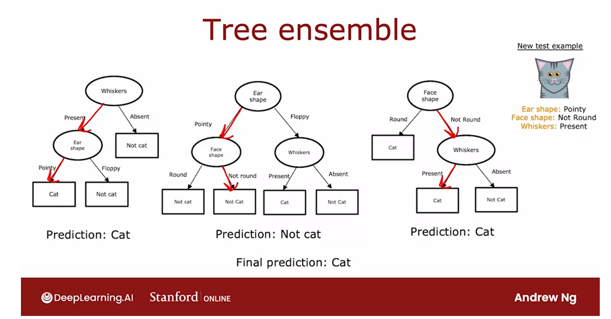
If you had this ensemble three trees, each one of these is maybe a plausible way to classify cat versus not cat.

We’ll see, in the
next few videos, how to construct this
ensemble of trees. But if you had this
ensemble three trees, each one of these is maybe a plausible way to classify
cat versus not cat.

If you had a new test example that you wanted to classify, then what you would do is run
all three of these trees on your new example and get them to vote on whether it’s
the final prediction.

This test example
has pointy ears, a not round face shape and
whiskers are present and so the first tree would
carry out inferences like this and predict
that it is a cat.

The second tree’s inference
would follow this path through the tree and therefore
predict that is not cat.

The third tree would
follow this path and therefore predict
that it is a cat.

Different trees have made different predictions and so what we’ll do is actually get them to vote.

These three trees have made different predictions and so what we’ll do is actually
get them to vote.

The majority votes
of the predictions among these three trees is, cat.

The final prediction of
this ensemble of trees is that this is a cat which happens to be the
correct prediction.

Tree ensembles: less sensitive and more robust

The reason we use an ensemble of trees is by having lots of decision trees and having them vote, it makes your overall algorithm less sensitive to what any single tree may be doing because it gets only one vote out of three or one vote out of many, many different votes and it makes your overall algorithm more robust.

The reason we use an
ensemble of trees is by having lots of decision trees and
having them vote, it makes your overall algorithm
less sensitive to what any single tree may
be doing because it gets only one vote out of
three or one vote out of many, many different
votes and it makes your overall algorithm
more robust.

But how do you come
up with all of these different plausible but maybe slightly different
decision trees in order to get them to vote?

In the next video, we’ll talk about
a technique from statistics called sampling with replacement and this will turn out to be a key
technique that we’ll use in the video after that in order to build this
ensemble of trees. Let’s go on to the
next video to talk about sampling with replacement.

Sampling with replacement

Sampling with replacement

In order to build
a tree ensemble, we’re going to need a technique called sampling
with replacement.

Let’s take a look
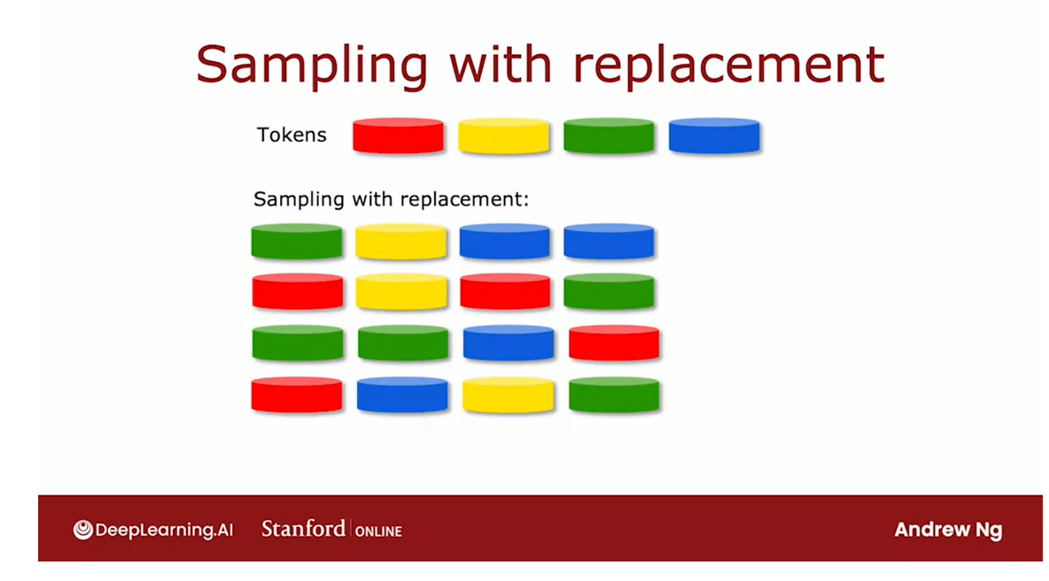
at what that means.

In order to illustrate how sampling with
replacement works, I’m going to show you a
demonstration of sampling with replacement using four
tokens that are colored red, yellow, green, and blue.

Example:

I actually have here with
me four tokens of colors, red, yellow, green, and blue. I’m going to demonstrate what sampling with replacement
using them look like. Here’s a black
velvet bag, empty.

I’m going to take this
example of four tokens, and drop them in. I’m going to sample four times with replacement
out of this bag.

What that means, I’m
going to shake it up, and can’t see when I’m picking, pick out one token,
turns out to be green.

Replacement: take out a token, put it back in and shake it up again, and then take on another one.

The term with replacement
means that if I take out the next token,
I’m going to take this, and put it back in,
and shake it up again, and then take on
another one, yellow.

Replace it. That’s a
little replacement part.

Then go again, blue
replace it again, and then pick on one more,
which is blue again.

That sequence of tokens I got was green, yellow, blue, blue.

Notice that I got blue twice, and didn’t get red
even a single time.

If you were to repeat
this sampling with replacement procedure
multiple times, if you were to do it again, you might get red, yellow, red, green, or green, green, blue, red. Or you might also get
red, blue, yellow, green.

Notice that the with replacement
part of this is critical because if I were not replacing a token
every time I sample, then if I were to pour four
tokens from my bag of four, I will always just get
the same four tokens.

That’s why replacing a token after I pull
it out each time, is important to
make sure I don’t just get the same four
tokens every single time.

The way that sampling
with replacement applies to building an ensemble
of trees is as follows.

Construct multiple random training sets

We are going to construct multiple random training sets that are all slightly different from our original training set.

In particular,
we’re going to take our 10 examples
of cats and dogs.

We’re going to put the
10 training examples in a theoretical bag. Please don’t actually put a
real cat or dog in a bag. That sounds inhumane,
but you can take a training example and put it in a theoretical
bag if you want.

I’m using this theoretical bag, we’re going to create a new random training set of 10 examples of the
exact same size as the original data set.

The way we’ll do so
is we’re reaching and pick out one random
training example.

Let’s say we get this
training example. Then we put it
back into the bag, and then again randomly pick out one training example
and so you get that.

You pick again and
again and again.

Notice now this fifth
training example is identical to the second
one that we had out there. But that’s fine.

You keep
going and keep going, and we get another
repeats the example, and so on and so forth.

Until eventually you end up
with 10 training examples, some of which are repeats.

You notice also that this
training set does not contain all 10 of the original training
examples, but that’s okay.

That is part of the sampling
with replacement procedure.

The process of sampling with replacement, lets you construct a new training set that’s a little bit similar to, but also pretty different from your original training set.

The process of sampling
with replacement, lets you construct
a new training set that’s a little bit similar to, but also pretty different from your original training set.

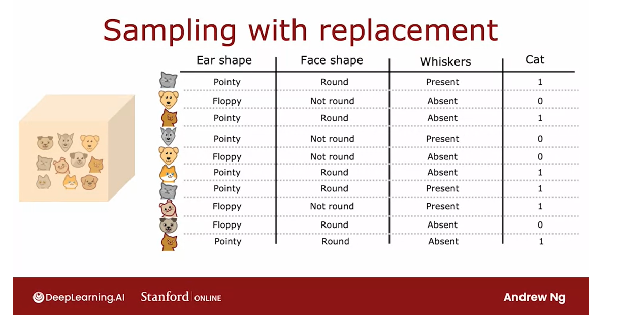
It turns out that this would be the key building block for
building an ensemble of trees. Let’s take a look
in the next video and how you could do that.

Random forest algorithm

Now that we have a way to use
something with replacement to create new training sets
that are a bit similar to but also quite different from
the original training set.

Random forest algorithm: powerful tree on sample algorithm

We’re ready to build our first
tree ensemble algorithm.

In particular in this video, we’ll talk about the random forest
algorithm which is one powerful tree on sample algorithm that works much better
than using a single decision tree.

Here’s how we can generate
an ensemble of trees.

If you are given a training set of size M,
then for b equals 1 to capital B so
we do this capital B times.

Put the M examples in a virtual bag and sample of replacement M times to generate a new training set

Then train a decision tree on this data set.

Go and repeat it again and again

You can use something with replacement
to create a new training set of size M.

So if you have 10 training examples,
you will put the 10 training examples in that virtual bag and sample of replacement
10 times to generate a new training set with also 10 examples, and then you would
train a decision tree on this data set.

So here’s the data set I’ve generated
using something with replacement.

If you look carefully, you may notice that some of the training
examples are repeated and that’s okay.

And if you train the decision on this data
said you end up with this decision tree.

Go and repeat it again and again

And having done this once, we would
then go and repeat this a second time.

Use something with replacement to
generate another training set of M or 10 training examples.

This again looks a bit like
the original training set but it’s also a little bit different.

You then train the decision
tree on this new data set and you end up with a somewhat
different decision tree. And so on.

And you may do this a total
of capital B times.

Typical choice of capital B the number
of such trees you built might be around a 100 people recommend
any value from Say 64, 228. And having built an ensemble
of say 100 different trees, you would then when you’re
trying to make a prediction, get these trees all votes on
the correct final prediction.

It turns out that setting capital B to be larger, never hurts performance, but beyond a certain point, you end up with diminishing returns and it doesn’t actually get that much better when B is much larger than say 100 or so.

It turns out that setting capital B to
be larger, never hurts performance, but beyond a certain point,
you end up with diminishing returns and it doesn’t actually get that much better
when B is much larger than say 100 or so.

Andrew: 不会用1000棵树

And that’s why I never use say 1000 trees
that just slows down the computation significantly without meaningfully
increasing the performance of the overall algorithm.

Bagged decision tree

放在袋子里的决策树：采用有放回采样得到新的数据集，然后训练决策树模型，重复B次，得到B棵决策树。

Just to give this particular algorithm name.

This specific instance creation of tree
ensemble is sometimes also called a bagged decision tree.

Bagged: that refers to putting your training examples in that virtual bag.

And that refers to putting your
training examples in that virtual bag.

And that’s why also we use the let
us lower case B an uppercase B here because that stands for bag.

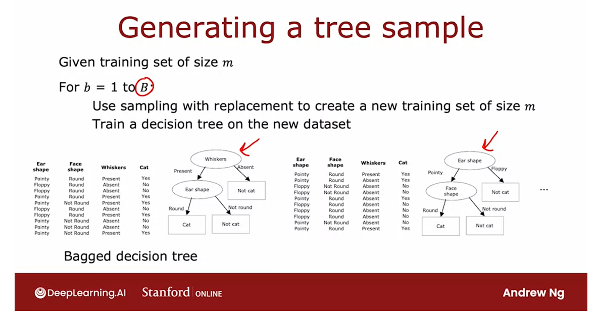
One modification: make it work even much better

There’s one modification to this algorithm
that will actually make it work even much better and that changes this algorithm the
back decision tree into the random forest algorithm.

有时候做切分的时候，结点所用的特征很多是重复的，这不好

The key idea is that even with this
sampling with replacement procedure sometimes you end up with always using
the same split at the root node and very similar splits near the root note.

That didn’t happen in this particular
example where a small change the trainings that resulted in a different
split at the root note.

But for other training sets it’s
not uncommon that for many or even all capital B training sets,
you end up with the same choice of feature at the root node and
at a few of the notes near the root note.

Randomize the feature choice at each node

So there’s one modification to
the algorithm to further try to randomize the feature choice at each note
that can cause the set of trees and you learn to become more
different from each other.

So when you vote them, you end up with
an even more accurate prediction.

The way this is typically done
is at every note when choosing a feature to use to slit if
end features are available.

So in our example we had three features
available rather than picking from all end features, we will instead pick a random
subset of K less than N features.

And allow the algorithm to choose
only from that subset of K features.

you would pick K less than N features as the allowed features and then out of those K features choose the one with the highest information gain as the choice of feature to use the split.

So in other words, you would pick K
features as the allowed features and then out of those K features
choose the one with the highest information gain as the choice
of feature to use the split.

When N is large, say n is Dozens or
10’s or even hundreds.

A typical choice for the value of K would be to choose it to be square root of N

A typical choice for the value of K would
be to choose it to be square root of N, In our example we have only three
features and this technique tends to be used more for larger problems
with a larger number of features.

And will just further change the algorithm
you end up with the random Forest algorithm which will work
typically much better and becomes much more robust than
just a single decision tree.

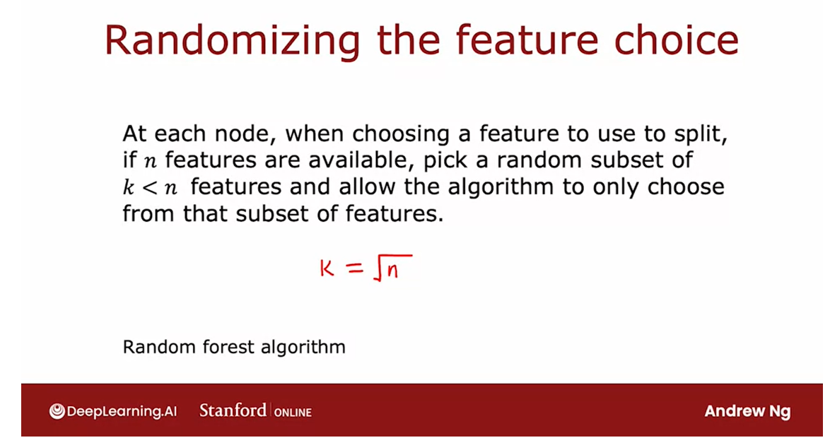
思考为什么这比单个决策树更稳健的一种方法是，带替换的程序使算法探索了对数据的许多小更改。算法正在训练不同的决策树，并对带替换的程序导致的所有数据更改进行平均。

One way to think about why this is more
robust to than a single decision tree is the something with replacement procedure
causes the algorithm to explore a lot of small changes to the data already and
it’s training different decision trees and is averaging over all of those
changes to the data that the something with replacement procedure causes.

因此，这意味着对训练集的任何微小更改都不太可能对整个随机森林算法的整体输出产生巨大影响。
因为已经对其进行了探索，并且对训练集进行了许多小的更改。

And so this means that any little change
further to the training set makes it less likely to have a huge impact on
the overall output of the overall random forest algorithm.

Because it’s already explored and it’s averaging over a lot of small
changes to the training set.

A joke

Q: Where does a machine learning engineer go camping?

A: In a random forest.

Andrew: All right. Go and tell that joke to your friends. I hope you enjoy it.

Before wrapping up this video there’s just
one more thought I want to share a view.

Which is, where does a machine
learning engineer go camping? In a random forest.

All right. Go and tell that joke to your friends. I hope you enjoy it.

The random forest is an effective our room
and I hope you better use it in your work. Beyond the random forest It turns out
there’s one other algorithm that works even better. Which is a boosted decision tree. In the next video, let’s talk about a boosted decision
tree algorithm called X G boost.

XGBoost

Today by far the most commonly used way or implementation of decision tree ensembles or decision trees there’s an algorithm called XGBoost.

Over the years, machine learning
researchers have come up with a lot of different ways to build decision trees and
decision tree on samples.

Today by far the most commonly used way or
implementation of decision tree ensembles or decision trees there’s
an algorithm called XGBoost.

It runs quickly, the open source
implementations are easily used, has also been used very successfully to
win many machine learning competitions as well as in many commercial applications.

Let’s take a look at how XGBoost works. There’s a modification to the back
decision tree algorithm that we saw in the last video that can
make it work much better.

Here again, is the algorithm that
we had written down previously.

Given the training set to size them,
you repeat B times, use something with replacement to
create a new training set of size M and then train the decision
tree on the new data set.

And so the first time through this loop, we may create a training set like that and
train a decision tree like that.

But here’s where we’re going to change the algorithm, which is every time through this loop, other than the first time, that is the second time, third time and so on.

When something rather than choosing each of the training examples with equal probability, we’re going to choose examples with higher probability that the ensemble of trees from the trees were built so far still gets wrong.

But here’s where we’re going to change
the algorithm, which is every time through this loop, other than the first time, that
is the second time, third time and so on.

When something rather than choosing
each of the training examples with equal probability, we’re going to
choose examples with higher probability that the ensemble of trees from the trees
were built so far still gets wrong.

Other than the first time through this loop, instead of picking from all examples of equal probability with one over m probability, let’s make it more likely that will pick examples that the previously trained trees misclassified or that the previously trained trees do poorly on.

But the second time through this loop,
instead of picking from all examples of equal probability
with one over m probability, let’s make it more likely that will pick
examples that the previously trained trees misclassified or that
the previously trained trees do poorly on.

类比：刻意练习 deliberate practice

Example: play the piano

In training and education, there’s
an idea called deliberate practice.

For example,
if you’re learning to play the piano and you’re trying to master a piece on the
piano rather than practicing the entire say five minute piece over and over,
which is quite time consuming.

If you instead play the piece and then focus your attention on just the parts of the piece that you aren’t yet playing that well in practice those smaller parts over and over.

Then that turns out to be a more efficient way for you to learn to play the piano well.

If you instead play the piece and then focus your attention on just
the parts of the piece that you aren’t yet playing that well in practice
those smaller parts over and over.

Then that turns out to be
a more efficient way for you to learn to play the piano well.

This idea of boosting is similar: deliberate practice

And so this idea of boosting is similar.

Look at what we’re not yet doing well on

We’re going to look at the decision trees,
we’ve trained so far and look at what we’re still not yet
doing well on.

And then when building
the next decision tree, we’re going to focus more attention on the
examples that we’re not yet doing well.

So rather than looking at all the training
examples, we focus more attention on the subset of examples is not yet doing
well on and get the new decision tree, the next decision tree reporting
ensemble to try to do well on them.

Boosting: help the learning algorithm learn to do better, more quickly

And this is the idea behind boosting and it turns out to help the learning
algorithm learn to do better more quickly.

So in detail, we will look at this
tree that we have just built and go back to the original training set.

Notice that this is
the original training set, not one generated through
something replacement.

And we’ll go through all ten examples and look at what this learned decision
tree predicts on all ten examples.

So this fourth most column
are their predictions and put a checkmark across
next to each example, depending on whether the trees
classification was correct or incorrect.

So what we’ll do in the second time
through this loop is we will sort of use something with replacement to generate
another training set of ten examples.

But every time we pick an example from these ten will give a higher chance of picking from one of these three examples that were still misclassifying.

But every time we pick an example from
these ten will give a higher chance of picking from one of these three examples
that were still misclassifying.

And so this focuses the second
decision trees attention via a process like deliberate practice on the examples
that the algorithm is still not yet doing that well.

And the boosting procedure
will do this for a total of B times where
on each iteration, you look at what the ensemble of trees for
trees 1, 2 up through (b- 1),
are not yet doing that well on.

And when you’re building tree number b, you will then have a higher
probability of picking examples that the ensemble of the previously sample
trees is still not yet doing well on.

The mathematical details of exactly
how much to increase the probability of picking this versus that
example are quite complex, but you don’t have to worry about them in
order to use russet tree implementations.

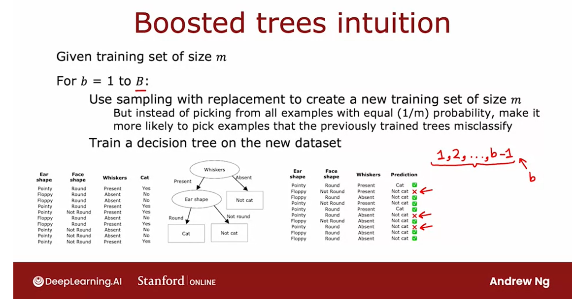
XGBoost： eXtreme Gradient Boosting = XGB

An open source implementation of boosted trees that is very fast and efficient

And of different ways of implementing
boosting the most widely used one today is XGBoost, which stands for extreme
gradient boosting, which is an open source implementation of boosted trees
that is very fast and efficient.

XGBoost also has a good choice of
the default splitting criteria and criteria for when to stop splitting.

And one of the innovations in
XGBoost is that it also has built in regularization to prevent overfitting,
and in machine learning competitions such as does a widely
used competition site called Kaggle.

XGBoost is often a highly
competitive algorithm.

XGBoost vs. Deep learning

In fact, XGBoost and deep learning
algorithms seem to be the two types of algorithms that win a lot
of these competitions.

And one technical note, rather than
doing something with replacement XGBoost actually assigns different ways
to different training examples.

So it doesn’t actually need to generate
a lot of randomly chosen training sets and this makes it even a little bit more
efficient than using a sampling with replacement procedure.

But the intuition that you saw on
the previous slide is still correct in terms of how XGBoost is
choosing examples to focus on.

The details of XGBoost are quite
complex to implement, which is why many practitioners will use the open source
libraries that implement XGBoost.

You’ll see and get your practice in detail using XGBoost
yourself in this week’s practice labs.

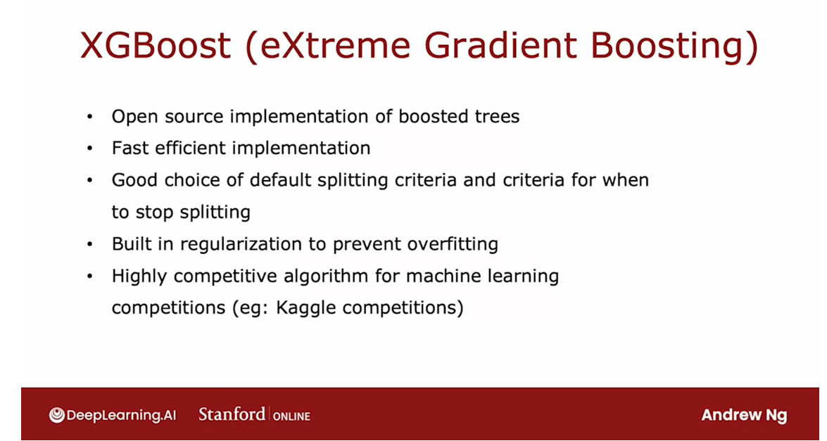
But very briefly, this is all you
need to do in order to use XGBoost, you will import the XGBoost
library as follows and initialize a model as
an XGBoost classifier.

Further model and then finally,
this allows you to make predictions using this boosted
decision trees algorithm.

I hope you have fun playing with this
in this week’s practice labs and they also find this algorithm useful for many applications that you
may build in the future.

Or alternatively, if you want to use
XGBoost for regression rather than for classification, then this line
here just becomes XGBRegressor and the rest of the code works similarly.

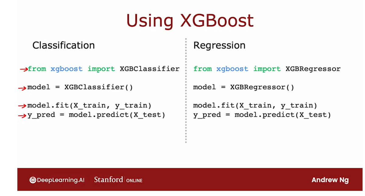
In the next video: Talk about when should you use a decision tree versus maybe use the neural network.

So that’s it for the XGBoost algorithm. We have just one last video for
this week and for this course where we’ll wrap up and also
talk about when should you use a decision tree versus maybe use the neural network.

Let’s go on to the last and
final video of this week.

When to use decision trees

Both decision trees, including tree ensembles as well as neural networks
are very powerful, very effective
learning algorithms.

When should you pick
one or the other?

Let’s look at some of the
pros and cons of each.

Pros and cons

Work well on tabular data: a giant spreadsheet

Decision trees and
tree ensembles will often work well on tabular data, also called structured data.

What that means is if
your dataset looks like a giant spreadsheet then decision trees would
be worth considering.

For example, in the housing price prediction
application we had a dataset with features corresponding to the
size of the house, the number of bedrooms,
the number of floors, and the age at home.

That type of data stored
in a spreadsheet with either categorical or continuous valued features and both for classification or for regression task where
you’re trying to predict a discrete category
or predict a number.

All of these problems are ones that decision trees
can do well on.

Decision trees work poorly on unstructured data

In contrast, I will
not recommend using decision trees and tree
ensembles on unstructured data.

That’s data such as
images, video, audio, and texts that you’re
less likely to store in a spreadsheet format.

Neural networks as we’ll see
in a second will tend to work better for
unstructured data task.

Can be very fast to train

One huge advantage of decision
trees and tree ensembles is that they can be
very fast to train.

You might remember this
diagram from the previous week in which we talked about the iterative loop of machine
learning development.

If your model takes many
hours to train then that limits how quickly
you can go through this loop and improve the
performance of your algorithm.

But because decision trees, including tree ensembles tend to be pretty fast to train, that allows you to go to
this loop more quickly and maybe more efficiently improve the performance of your
learning algorithm.

Small decision trees maybe human interpretable

Finally, small decision trees
maybe human interpretable.

If you are training just
a single decision tree and that decision
tree has only say a few dozen notes you
may be able to print out a decision tree to understand exactly how
it’s making decisions.

I think that the
interpretability of decision trees is
sometimes a bit overstated because when you
build an ensemble of 100 trees and if each of those trees has
hundreds of nodes, then looking at that ensemble
to figure out what it’s doing does become difficult and may need some separate
visualization techniques.

But if you have a small
decision tree you can actually look at it and see, oh, it’s classifying whether
something is a cut by looking at certain
features in certain ways.

If you’ve decided to use a decision tree or tree ensemble, I would probably use XGBoost for most of the applications I will work on.

If you’ve decided to use a decision tree
or tree ensemble, I would probably use XGBoost for most of the
applications I will work on.

One slight downside of tree ensemble: a bit more expensive

One slight downside of a
tree ensemble is that it is a bit more expensive than
a single decision tree.

If you had a very constrained
computational budget you might use a
single decision tree but other than that setting
I would almost always use a tree ensemble and
use XGBoost in particular.

上面介绍决策树和决策树群的优缺点，下面主要关于神经网络

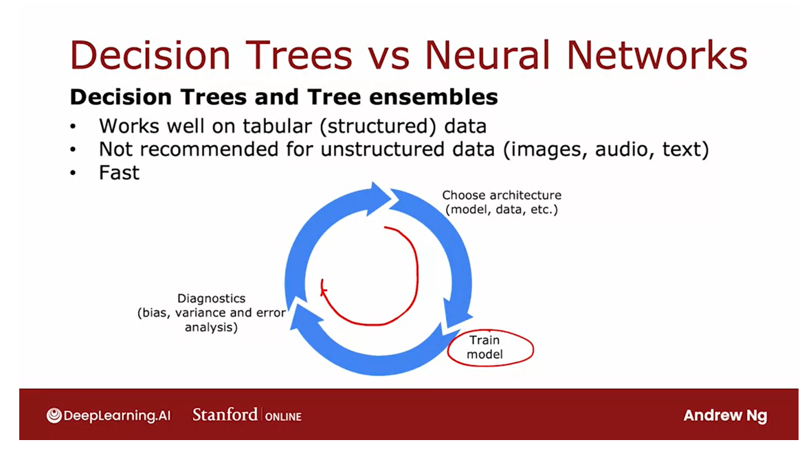
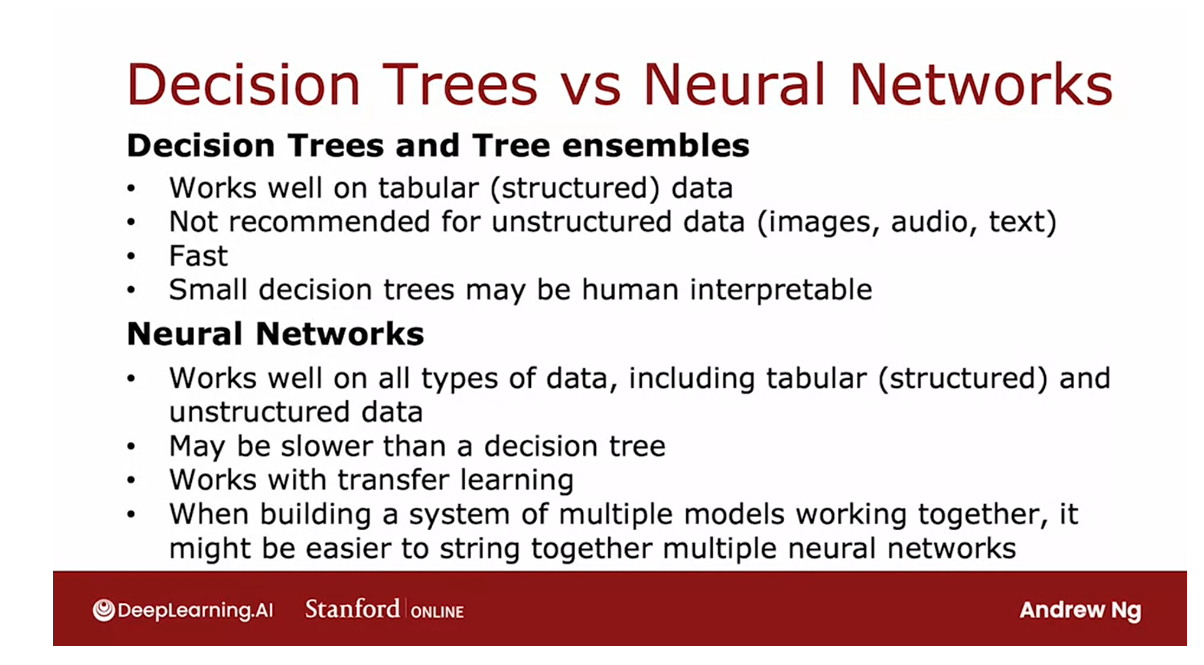
How about neural networks?

In contrast to decision
trees and tree ensembles, it works well on
all types of data, including tabular or structured data as well as
unstructured data.

As well as mixed
data that includes both structured and
unstructured components.

Neural network: on unstructured data, such as images, video, audio, and text, a neural network will really be the preferred algorithm and not the decision tree or a tree ensemble.

Whereas on tabular
structured data, neural networks and decision
trees are often both competitive on unstructured
data, such as images, video, audio, and text, a neural network will really be the preferred algorithm and not the decision tree
or a tree ensemble.

On the downside though, neural networks may be
slower than a decision tree.

A large neural network can just take a long time to train.

Other benefits of neural
networks includes that it works with transfer
learning and this is really important because
for many applications we have only a small
dataset being able to use transfer learning and
carry out pre-training on a much larger dataset that is critical to getting
competitive performance.

Finally, there are also some technical reasons
why it might be easier to string together multiple
neural networks to build a larger
machine learning system.

NN compute the output y as a smooth or continuous function of the input x

String together a lot of different models, the outputs are differentiable

Train them all at the same time using gradient descent.

The basic reason is neural
networks compute the output y as a smooth or
continuous function of the input x and so even if you string
together a lot of different models the
outputs of all of these different models is
itself differentiable and so you can train them all at the same time using
gradient descent.

Whereas with a decision tree you can only train one tree at a time.

Whereas with a decision
tree you can only train one tree at a time.

Finally, if you’re
building a system of multiple machine learning
models working together, it might be easier to
string together and train multiple neural networks than multiple decision trees.

The reasons for this are
quite technical and you don’t need to worry about it for the purpose
of this course.

But it relates to that even when you string together
multiple neural networks you can train them all together
using gradient descent.

Whereas for decision
trees you can only train one decision tree at
a time.

Reached the end of the video

That’s it. You’ve reached the
end of the videos for this course on Advanced
Learning Algorithms.

Thank you for sticking
with me all this way and congratulations
on getting to the end of the videos on
advanced learning algorithms.

Wrap up

You’ve now learned how to build and use both
neural networks and decision trees and also heard about a variety of tips, practical advice on how to get these algorithms to
work well for you.

But even if all that you’ve
seen on supervised learning, that’s just part of what
learning algorithms can do.

Supervised learnings
need labeled datasets with the labels Y on
your training set.

There’s another set of
very powerful algorithms called unsupervised
learning algorithms where you don’t even need labels Y for the
algorithm to figure out very interesting patterns and to do things with the
data that you have.

I look forward to
seeing you also in the third and final course of this specialization which should be on unsupervised learning.

Now, before you
finish up this course I hope you also enjoy practicing the ideas of decision trees in their practice quizzes and
in their practice labs.

I’d like to wish you
the best of luck in the practice labs or for those of you that may
be Star Wars fans, let me say, may the
forest be with you.

[6] Practice quiz: Tree ensembles

Practice quiz: Tree ensembles

Latest Submission Grade 100%

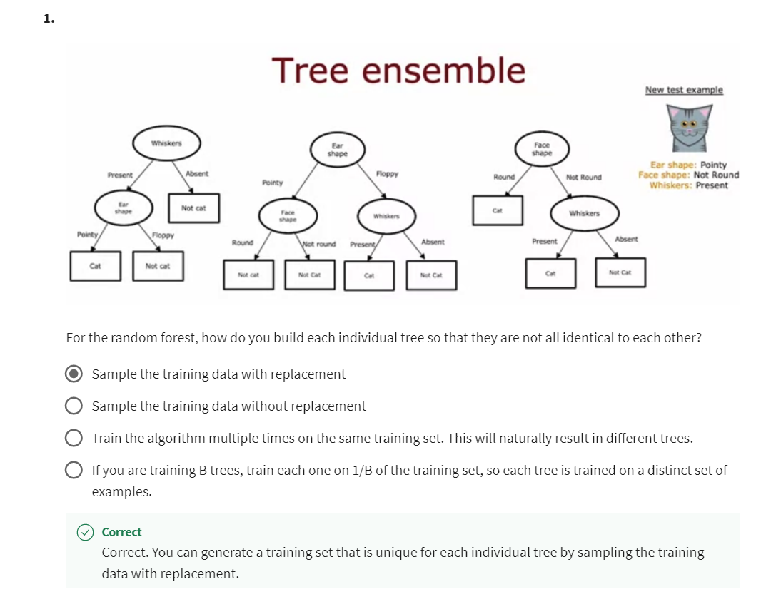
Correct. You can generate a training set that is unique for each individual tree by sampling the training data with replacement.

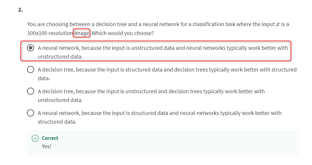
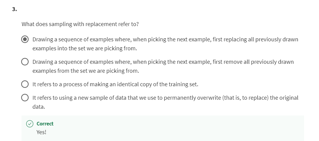
行百里者半九十

2022年7月2日22点22分这节课的进度如下：

[7] Practice lab: decision trees

Welcome to the last practice lab of this course. In this exercise, you will implement a decision tree from scratch and apply it to the task of classifying whether a mushroom is edible or poisonous.

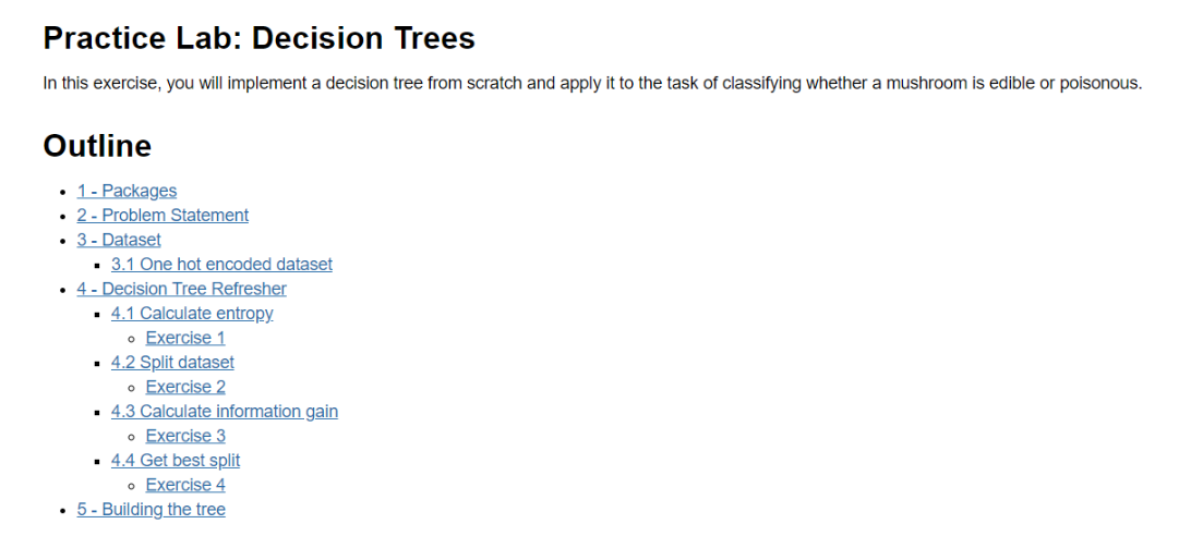
Practice Lab: Decision Trees

In this exercise, you will implement a decision tree from scratch and apply it to the task of classifying whether a mushroom is edible or poisonous.

1 - Packages

First, let’s run the cell below to import all the packages that you will need during this assignment.

• numpy is the fundamental package for working with matrices in Python.
• matplotlib is a famous library to plot graphs in Python.
• utils.py contains helper functions for this assignment. You do not need to modify code in this file.

import numpy as np
import matplotlib.pyplot as plt
from public_tests import *

%matplotlib inline

2 - Problem Statement

Suppose you are starting a company that grows and sells wild mushrooms.

• Since not all mushrooms are edible, you’d like to be able to tell whether a given mushroom is edible or poisonous based on it’s physical attributes
• You have some existing data that you can use for this task.

Can you use the data to help you identify which mushrooms can be sold safely?

Note: The dataset used is for illustrative purposes only. It is not meant to be a guide on identifying edible mushrooms.

3 - Dataset

stalk shape: 茎秆形状

You will start by loading the dataset for this task. The dataset you have collected is as follows:

Cap Color	Stalk Shape	Solitary	Edible
Brown	Tapering	Yes	1
Brown	Enlarging	Yes	1
Brown	Enlarging	No	0
Brown	Enlarging	No	0
Brown	Tapering	Yes	1
Red	Tapering	Yes	0
Red	Enlarging	No	0
Brown	Enlarging	Yes	1
Red	Tapering	No	1
Brown	Enlarging	No	0

• You have 10 examples of mushrooms. For each example, you have
  • Three features
    • Cap Color (Brown or Red),
    • Stalk Shape (Tapering or Enlarging), and
    • Solitary (Yes or No)
  • Label
    • Edible (1 indicating yes or 0 indicating poisonous)

3.1 One hot encoded dataset

For ease of implementation, we have one-hot encoded the features (turned them into 0 or 1 valued features)

Brown Cap	Tapering Stalk Shape	Solitary	Edible
1	1	1	1
1	0	1	1
1	0	0	0
1	0	0	0
1	1	1	1
0	1	1	0
0	0	0	0
1	0	1	1
0	1	0	1
1	0	0	0

Therefore,

• X_train contains three features for each example
  • Brown Color (A value of 1 indicates “Brown” cap color and 0 indicates “Red” cap color)
  • Tapering Shape (A value of 1 indicates “Tapering Stalk Shape” and 0 indicates “Enlarging” stalk shape) 锥形形状（“1”表示“锥形茎形状”，“0”表示“扩大”茎形状）
  • Solitary (A value of 1 indicates “Yes” and 0 indicates “No”)
• y_train is whether the mushroom is edible
  • y = 1 indicates edible
  • y = 0 indicates poisonous

X_train = np.array([[1,1,1],[1,0,1],[1,0,0],[1,0,0],[1,1,1],[0,1,1],[0,0,0],[1,0,1],[0,1,0],[1,0,0]])
y_train = np.array([1,1,0,0,1,0,0,1,1,0])

View the variables

Let’s get more familiar with your dataset.

• A good place to start is to just print out each variable and see what it contains.

The code below prints the first few elements of X_train and the type of the variable.

print("First few elements of X_train:\n", X_train[:5])
print("Type of X_train:",type(X_train))

Output

First few elements of X_train:
 [[1 1 1]
 [1 0 1]
 [1 0 0]
 [1 0 0]
 [1 1 1]]
Type of X_train: <class 'numpy.ndarray'>

Now, let’s do the same for y_train

print("First few elements of y_train:", y_train[:5])
print("Type of y_train:",type(y_train))

Output

First few elements of y_train: [1 1 0 0 1]
Type of y_train: <class 'numpy.ndarray'>

Check the dimensions of your variables

Another useful way to get familiar with your data is to view its dimensions.

Please print the shape of X_train and y_train and see how many training examples you have in your dataset.

print ('The shape of X_train is:', X_train.shape)
print ('The shape of y_train is: ', y_train.shape)
print ('Number of training examples (m):', len(X_train))

Output

The shape of X_train is: (10, 3)
The shape of y_train is:  (10,)
Number of training examples (m): 10

4 - Decision Tree Refresher

In this practice lab, you will build a decision tree based on the dataset provided.

• Recall that the steps for building a decision tree are as follows:

  • Start with all examples at the root node
  • Calculate information gain for splitting on all possible features, and pick the one with the highest information gain
  • Split dataset according to the selected feature, and create left and right branches of the tree
  • Keep repeating splitting process until stopping criteria is met

• In this lab, you’ll implement the following functions, which will let you split a node into left and right branches using the feature with the highest information gain

  • Calculate the entropy at a node
  • Split the dataset at a node into left and right branches based on a given feature
  • Calculate the information gain from splitting on a given feature
  • Choose the feature that maximizes information gain

• We’ll then use the helper functions you’ve implemented to build a decision tree by repeating the splitting process until the stopping criteria is met

  • For this lab, the stopping criteria we’ve chosen is setting a maximum depth of 2

4.1 Calculate entropy

First, you’ll write a helper function called compute_entropy that computes the entropy (measure of impurity) at a node.

• The function takes in a numpy array (y) that indicates whether the examples in that node are edible (1) or poisonous(0)

Complete the compute_entropy() function below to:

• Compute $p_1$, which is the fraction of examples that are edible (i.e. have value = 1 in y)
• The entropy is then calculated as

$$H(p_1)=-p_1{\text{log}}_2(p_1)-(1-p_1){\text{log}}_2(1-p_1)$$

• Note
  • The log is calculated with base $2$
  • For implementation purposes, $0{\text{log}}_2(0)=0$. That is, if p_1 = 0 or p_1 = 1, set the entropy to 0
  • Make sure to check that the data at a node is not empty (i.e. len(y) != 0). Return 0 if it is

Exercise 1

Please complete the compute_entropy() function using the previous instructions.

If you get stuck, you can check out the hints presented after the cell below to help you with the implementation.

The first try

# UNQ_C1
# GRADED FUNCTION: compute_entropy

def compute_entropy(y):
    """
    Computes the entropy for 
    
    Args:
       y (ndarray): Numpy array indicating whether each example at a node is
           edible (`1`) or poisonous (`0`)
       
    Returns:
        entropy (float): Entropy at that node
        
    """
    # You need to return the following variables correctly
    entropy = 0.
    
    ### START CODE HERE ###
    y_length = len(y)
    
    if y_length == 0:
        return 0
    
    num_of_edible = 0
    for i in range(y_length):
        if y[i] == 1:
            num_of_edible += 1
    
    p1 = 0.
    p1 = num_of_edible / y_length
    
    entropy = -(p1 * np.log2(p1) + (1 - p1) * np.log2(1 - p1))
           
    ### END CODE HERE ###        
    
    return entropy

Unit test ERROR

---------------------------------------------------------------------------
AssertionError                            Traceback (most recent call last)
<ipython-input-9-05098bb5d0e3> in <module>
      5 
      6 # UNIT TESTS
----> 7 compute_entropy_test(compute_entropy)

~/work/public_tests.py in compute_entropy_test(target)
      5     result = target(y)
      6 
----> 7     assert result == 0, "Entropy must be 0 with array of ones"
      8 
      9     y = np.array([0] * 10)

AssertionError: Entropy must be 0 with array of ones

Summary: lack of checking p1 if equals 0 or 1

The second try: pass the tests

And NOT the latest version

# UNQ_C1
# GRADED FUNCTION: compute_entropy

def compute_entropy(y):
    """
    Computes the entropy for 
    
    Args:
       y (ndarray): Numpy array indicating whether each example at a node is
           edible (`1`) or poisonous (`0`)
       
    Returns:
        entropy (float): Entropy at that node
        
    """
    # You need to return the following variables correctly
    entropy = 0.
    
    ### START CODE HERE ###
    y_length = len(y)
    
    if y_length == 0:
        return 0
    
    num_of_edible = 0
    for i in range(y_length):
        if y[i] == 1:
            num_of_edible += 1
    
    p1 = 0.
    p1 = num_of_edible / y_length # correct answer, my solution
    
    # optimize
    # p1 = len(y[y == 1]) / len(y)
    
    if p1 == 0 or p1 == 1:
        return 0
    
    entropy = -p1 * np.log2(p1) - (1 - p1) * np.log2(1 - p1)
           
    ### END CODE HERE ###        
    
    return entropy

You can check if your implementation was correct by running the following test code:

# Compute entropy at the root node (i.e. with all examples)
# Since we have 5 edible and 5 non-edible mushrooms, the entropy should be 1"

print("Entropy at root node: ", compute_entropy(y_train)) 

# UNIT TESTS
compute_entropy_test(compute_entropy)

Output

Entropy at root node:  1.0
 All tests passed.

Hints

• To calculate p1
  • You can get the subset of examples in y that have the value 1 as y[y == 1]
  • You can use len(y) to get the number of examples in y
• To calculate entropy
  • np.log2 let’s you calculate the logarithm to base 2 for a numpy array
  • If the value of p1 is 0 or 1, make sure to set the entropy to 0

More hints

Here’s how you can structure the overall implementation for this function

def compute_entropy(y):

 # You need to return the following variables correctly
 entropy = 0.

 ### START CODE HERE ###
 if len(y) != 0:
     # Your code here to calculate the fraction of edible examples (i.e with value = 1 in y)
     p1 =

     # For p1 = 0 and 1, set the entropy to 0 (to handle 0log0)
     if p1 != 0 and p1 != 1:
         # Your code here to calculate the entropy using the formula provided above
         entropy = 
     else:
         entropy = 0. 
 ### END CODE HERE ###        

 return entropy

If you’re still stuck, you can check the hints presented below to figure out how to calculate p1 and entropy.

You can compute p1 as p1 = len(y[y == 1]) / len(y)

You can compute entropy as entropy = -p1 * np.log2(p1) - (1 - p1) * np.log2(1 - p1)

The latest version of code

# UNQ_C1
# GRADED FUNCTION: compute_entropy

def compute_entropy(y):
    """
    Computes the entropy for 
    
    Args:
       y (ndarray): Numpy array indicating whether each example at a node is
           edible (`1`) or poisonous (`0`)
       
    Returns:
        entropy (float): Entropy at that node
        
    """
    # You need to return the following variables correctly
    entropy = 0.
    
    ### START CODE HERE ###
    
    if len(y) == 0:
        return 0

    # optimize
    p1 = len(y[y == 1]) / len(y)
    
    if p1 == 0 or p1 == 1:
        return 0
    
    entropy = -p1 * np.log2(p1) - (1 - p1) * np.log2(1 - p1)
           
    ### END CODE HERE ###        
    
    return entropy

Expected Output:

Entropy at root node: 1.0

4.2 Split dataset

Next, you’ll write a helper function called split_dataset that takes in the data at a node and a feature to split on and splits it into left and right branches. Later in the lab, you’ll implement code to calculate how good the split is.

• The function takes in the training data, the list of indices of data points at that node, along with the feature to split on.
• It splits the data and returns the subset of indices at the left and the right branch.
• For example, say we’re starting at the root node (so node_indices = [0,1,2,3,4,5,6,7,8,9]), and we chose to split on feature 0, which is whether or not the example has a brown cap.
  • The output of the function is then, left_indices = [0,1,2,3,4,7,9] and right_indices = [5,6,8]

Index	Brown Cap	Tapering Stalk Shape	Solitary	Edible
0	1	1	1	1
1	1	0	1	1
2	1	0	0	0
3	1	0	0	0
4	1	1	1	1
5	0	1	1	0
6	0	0	0	0
7	1	0	1	1
8	0	1	0	1
9	1	0	0	0

Exercise 2

Please complete the split_dataset() function shown below

• For each index in node_indices
  • If the value of X at that index for that feature is 1, add the index to left_indices
  • If the value of X at that index for that feature is 0, add the index to right_indices

If you get stuck, you can check out the hints presented after the cell below to help you with the implementation.

My try: ERROR

# UNQ_C2
# GRADED FUNCTION: split_dataset

def split_dataset(X, node_indices, feature):
    """
    Splits the data at the given node into
    left and right branches
    
    Args:
        X (ndarray):             Data matrix of shape(n_samples, n_features)
        node_indices (ndarray):  List containing the active indices. I.e, the samples being considered at this step.
        feature (int):           Index of feature to split on
    
    Returns:
        left_indices (ndarray): Indices with feature value == 1
        right_indices (ndarray): Indices with feature value == 0
    """
    
    # You need to return the following variables correctly
    left_indices = []
    right_indices = []
    
    ### START CODE HERE ###
    len_of_indices = len(node_indices)
    
    #print(X[2, :])
    for i in range(len_of_indices):
        if X[i][feature] == 1:
            left_indices.append(i)
        elif X[i][feature] == 0:
            right_indices.append(i)
           
    ### END CODE HERE ###
        
    return left_indices, right_indices

Output

ValueError: operands could not be broadcast together with shapes (3,) (4,) 

After checking out the hints, my code passed all the tests.

Directly use for i in node_indices:, instead of using range(0, len(node_indices))

# UNQ_C2
# GRADED FUNCTION: split_dataset

def split_dataset(X, node_indices, feature):
    """
    Splits the data at the given node into
    left and right branches
    
    Args:
        X (ndarray):             Data matrix of shape(n_samples, n_features)
        node_indices (ndarray):  List containing the active indices. I.e, the samples being considered at this step.
        feature (int):           Index of feature to split on
    
    Returns:
        left_indices (ndarray): Indices with feature value == 1
        right_indices (ndarray): Indices with feature value == 0
    """
    
    # You need to return the following variables correctly
    left_indices = []
    right_indices = []
    
    ### START CODE HERE ###
    for i in node_indices:
        if X[i][feature] == 1:
            left_indices.append(i)
        elif X[i][feature] == 0:
            right_indices.append(i)
           
    ### END CODE HERE ###
        
    return left_indices, right_indices

Now, let’s check your implementation using the code blocks below. Let’s try splitting the dataset at the root node, which contains all examples at feature 0 (Brown Cap) as we’d discussed above

root_indices = [0, 1, 2, 3, 4, 5, 6, 7, 8, 9]

# Feel free to play around with these variables
# The dataset only has three features, so this value can be 0 (Brown Cap), 1 (Tapering Stalk Shape) or 2 (Solitary)
feature = 0

left_indices, right_indices = split_dataset(X_train, root_indices, feature)

print("Left indices: ", left_indices)
print("Right indices: ", right_indices)

# UNIT TESTS    
split_dataset_test(split_dataset)

Output

Left indices:  [0, 1, 2, 3, 4, 7, 9]
Right indices:  [5, 6, 8]
 All tests passed.

Expected Output:

Left indices:  [0, 1, 2, 3, 4, 7, 9]
Right indices:  [5, 6, 8]

Hints

Here’s how you can structure the overall implementation for this function

def split_dataset(X, node_indices, feature):

   # You need to return the following variables correctly
   left_indices = []
   right_indices = []

   ### START CODE HERE ###
   # Go through the indices of examples at that node
   for i in node_indices:   
       if # Your code here to check if the value of X at that index for the feature is 1
           left_indices.append(i)
       else:
           right_indices.append(i)
   ### END CODE HERE ###

return left_indices, right_indices

More hints

The condition is if X[i][feature] == 1:.

4.3 Calculate information gain

Next, you’ll write a function called information_gain that takes in the training data, the indices at a node and a feature to split on and returns the information gain from the split.

Exercise 3

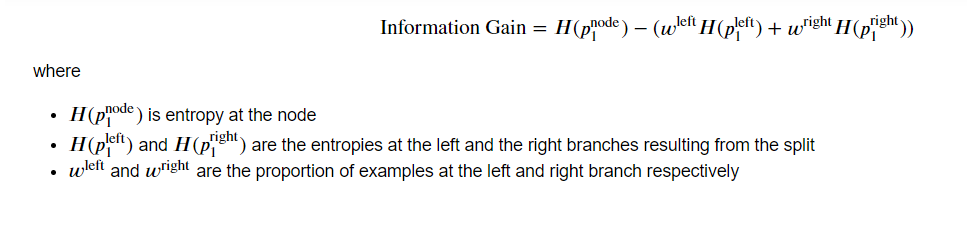
Please complete the compute_information_gain() function shown below to compute

$$\text{Information Gain}=H(p_1^{\text{node}})-(w^{\text{left}}H(p_1^{\text{left}})+w^{\text{right}}H(p_1^{\text{right}}))$$

where

• $H(p_1^{\text{node}})$ is entropy at the node
• $H(p_1^{\text{left}})$ and $H(p_1^{\text{right}})$ are the entropies at the left and the right branches resulting from the split
• $w^{\text{left}}$ and $w^{\text{right}}$ are the proportion of examples at the left and right branch respectively

Note:

• You can use the compute_entropy() function that you implemented above to calculate the entropy
• We’ve provided some starter code that uses the split_dataset() function you implemented above to split the dataset

If you get stuck, you can check out the hints presented after the cell below to help you with the implementation.

My try: ERROR

Instead of using compute_entropy(y), I should use compute_entropy(y_node)

# UNQ_C3
# GRADED FUNCTION: compute_information_gain

def compute_information_gain(X, y, node_indices, feature):
    
    """
    Compute the information of splitting the node on a given feature
    
    Args:
        X (ndarray):            Data matrix of shape(n_samples, n_features)
        y (array like):         list or ndarray with n_samples containing the target variable
        node_indices (ndarray): List containing the active indices. I.e, the samples being considered in this step.
   
    Returns:
        cost (float):        Cost computed
    
    """    
    # Split dataset
    left_indices, right_indices = split_dataset(X, node_indices, feature)
    
    # Some useful variables
    X_node, y_node = X[node_indices], y[node_indices]
    X_left, y_left = X[left_indices], y[left_indices]
    X_right, y_right = X[right_indices], y[right_indices]
    
    # You need to return the following variables correctly
    information_gain = 0
    print(f'y_node: {y_node}')
    print(f'y_left: {y_left}')
    
    ### START CODE HERE ###
    
    # Weights 
    w_left = len(y_left) / len(y_node)
    w_right = len(y_right) / len(y_node)
    
    #Weighted entropy
    h_of_node = compute_entropy(y)
    h_of_left = compute_entropy(y_left)
    h_of_right = compute_entropy(y_right)
     
    #Information gain                                                   
    information_gain = h_of_node - (w_left * h_of_left + w_right * h_of_right)
    
    ### END CODE HERE ###  
    
    return information_gain

Output

~/work/public_tests.py in compute_information_gain_test(target)
    101     node_indexes = list(range(4))
    102     result = target(X, y, node_indexes, 0)
--> 103     assert np.isclose(result, 0.311278, atol=1e-6), f"Wrong information gain. Expected {0.311278} got: {result}"
    104 
    105     result = target(X, y, node_indexes, 1)

AssertionError: Wrong information gain. Expected 0.311278 got: 0.2822287189138014

Refactor my code

# UNQ_C3
# GRADED FUNCTION: compute_information_gain

def compute_information_gain(X, y, node_indices, feature):
    
    """
    Compute the information of splitting the node on a given feature
    
    Args:
        X (ndarray):            Data matrix of shape(n_samples, n_features)
        y (array like):         list or ndarray with n_samples containing the target variable
        node_indices (ndarray): List containing the active indices. I.e, the samples being considered in this step.
   
    Returns:
        cost (float):        Cost computed
    
    """    
    # Split dataset
    left_indices, right_indices = split_dataset(X, node_indices, feature)
    
    # Some useful variables
    X_node, y_node = X[node_indices], y[node_indices]
    X_left, y_left = X[left_indices], y[left_indices]
    X_right, y_right = X[right_indices], y[right_indices]
    
    # You need to return the following variables correctly
    information_gain = 0
    print(f'y_node: {y_node}')
    print(f'y_left: {y_left}')
    
    ### START CODE HERE ###
    
    # Weights 
    w_left = len(y_left) / len(y_node)
    w_right = len(y_right) / len(y_node)
    
    #Weighted entropy
    h_of_node = compute_entropy(y_node)  # <---- fix a bug here
    h_of_left = compute_entropy(y_left)
    h_of_right = compute_entropy(y_right)
     
    #Information gain                                                   
    information_gain = h_of_node - (w_left * h_of_left + w_right * h_of_right)
    
    ### END CODE HERE ###  
    
    return information_gain

Carry out unit test and pass all the tests.

You can now check your implementation using the cell below and calculate what the information gain would be from splitting on each of the features

Unit test

info_gain0 = compute_information_gain(X_train, y_train, root_indices, feature=0)
print("Information Gain from splitting the root on brown cap: ", info_gain0)
    
info_gain1 = compute_information_gain(X_train, y_train, root_indices, feature=1)
print("Information Gain from splitting the root on tapering stalk shape: ", info_gain1)

info_gain2 = compute_information_gain(X_train, y_train, root_indices, feature=2)
print("Information Gain from splitting the root on solitary: ", info_gain2)

# UNIT TESTS
compute_information_gain_test(compute_information_gain)

Output

Information Gain from splitting the root on brown cap:  0.034851554559677034
Information Gain from splitting the root on tapering stalk shape:  0.12451124978365313
Information Gain from splitting the root on solitary:  0.2780719051126377
 All tests passed.

Expected Output:

Information Gain from splitting the root on brown cap:  0.034851554559677034
Information Gain from splitting the root on tapering stalk shape:  0.12451124978365313
Information Gain from splitting the root on solitary:  0.2780719051126377

Splitting on “Solitary” (feature = 2) at the root node gives the maximum information gain. Therefore, it’s the best feature to split on at the root node.

Hints

Here’s how you can structure the overall implementation for this function

def compute_information_gain(X, y, node_indices, feature):
   # Split dataset
   left_indices, right_indices = split_dataset(X, node_indices, feature)

   # Some useful variables
   X_node, y_node = X[node_indices], y[node_indices]
   X_left, y_left = X[left_indices], y[left_indices]
   X_right, y_right = X[right_indices], y[right_indices]

   # You need to return the following variables correctly
   information_gain = 0

   ### START CODE HERE ###
   # Your code here to compute the entropy at the node using compute_entropy()
   node_entropy = 
   # Your code here to compute the entropy at the left branch
   left_entropy = 
   # Your code here to compute the entropy at the right branch
   right_entropy = 

   # Your code here to compute the proportion of examples at the left branch
   w_left = 

   # Your code here to compute the proportion of examples at the right branch
   w_right = 

   # Your code here to compute weighted entropy from the split using 
   # w_left, w_right, left_entropy and right_entropy
   weighted_entropy = 

   # Your code here to compute the information gain as the entropy at the node
   # minus the weighted entropy
   information_gain = 
   ### END CODE HERE ###  

   return information_gain

More hints

node_entropy = compute_entropy(y_node)
left_entropy = compute_entropy(y_left)
right_entropy = compute_entropy(y_right)

w_left = len(X_left) / len(X_node)
w_right = len(X_right) / len(X_node)

weighted_entropy = w_left * left_entropy + w_right * right_entropy

information_gain = node_entropy - weighted_entropy

After reading the hints, just refactor my code

A refined version

# UNQ_C3
# GRADED FUNCTION: compute_information_gain

def compute_information_gain(X, y, node_indices, feature):
    
    """
    Compute the information of splitting the node on a given feature
    
    Args:
        X (ndarray):            Data matrix of shape(n_samples, n_features)
        y (array like):         list or ndarray with n_samples containing the target variable
        node_indices (ndarray): List containing the active indices. I.e, the samples being considered in this step.
   
    Returns:
        cost (float):        Cost computed
    
    """    
    # Split dataset
    left_indices, right_indices = split_dataset(X, node_indices, feature)
    
    # Some useful variables
    X_node, y_node = X[node_indices], y[node_indices]
    X_left, y_left = X[left_indices], y[left_indices]
    X_right, y_right = X[right_indices], y[right_indices]
    
    # You need to return the following variables correctly
    information_gain = 0
    
    ### START CODE HERE ###
    
    # Weights 
    w_left = len(y_left) / len(y_node)
    w_right = len(y_right) / len(y_node)
    
    #Weighted entropy
    node_entropy = compute_entropy(y_node)
    left_entropy = compute_entropy(y_left)
    right_entropy = compute_entropy(y_right)
    
    weighted_entropy = w_left * left_entropy + w_right * right_entropy
     
    #Information gain                                                   
    information_gain = node_entropy - weighted_entropy
    
    ### END CODE HERE ###  
    
    return information_gain

4.4 Get best split

Now let’s write a function to get the best feature to split on by computing the information gain from each feature as we did above and returning the feature that gives the maximum information gain

Exercise 4

Please complete the get_best_split() function shown below.

• The function takes in the training data, along with the indices of datapoint at that node
• The output of the function: the feature that gives the maximum information gain
  • You can use the compute_information_gain() function to iterate through the features and calculate the information for each feature

If you get stuck, you can check out the hints presented after the cell below to help you with the implementation.

My code: pass all the tests

# UNQ_C4
# GRADED FUNCTION: get_best_split

def get_best_split(X, y, node_indices):   
    """
    Returns the optimal feature and threshold value
    to split the node data 
    
    Args:
        X (ndarray):            Data matrix of shape(n_samples, n_features)
        y (array like):         list or ndarray with n_samples containing the target variable
        node_indices (ndarray): List containing the active indices. I.e, the samples being considered in this step.

    Returns:
        best_feature (int):     The index of the best feature to split
    """    
    
    # Some useful variables
    num_features = X.shape[1]
    
    # You need to return the following variables correctly
    best_feature = -1
    
    ### START CODE HERE ###
    max_information_gain = 0
    for feature in range(num_features):
        information_gain_of_feature_i = compute_information_gain(X, y, node_indices, feature)
        
        if information_gain_of_feature_i > max_information_gain:
            max_information_gain = information_gain_of_feature_i
            best_feature = feature
       
    ### END CODE HERE ##    
   
    return best_feature

Now, let’s check the implementation of your function using the cell below.

best_feature = get_best_split(X_train, y_train, root_indices)
print("Best feature to split on: %d" % best_feature)

# UNIT TESTS
get_best_split_test(get_best_split)

Output

Best feature to split on: 2
 All tests passed.

As we saw above, the function returns that the best feature to split on at the root node is feature 2 (“Solitary”)

Hints

Here’s how you can structure the overall implementation for this function

def get_best_split(X, y, node_indices):   

   # Some useful variables
   num_features = X.shape[1]

   # You need to return the following variables correctly
   best_feature = -1

   ### START CODE HERE ###
   max_info_gain = 0

   # Iterate through all features
   for feature in range(num_features): 

       # Your code here to compute the information gain from splitting on this feature
       info_gain = 

       # If the information gain is larger than the max seen so far
       if info_gain > max_info_gain:  
           # Your code here to set the max_info_gain and best_feature
           max_info_gain = 
           best_feature = 
   ### END CODE HERE ##    

return best_feature

More hints

info_gain = compute_information_gain(X, y, node_indices, feature)

max_info_gain = info_gain
best_feature = feature

After reading the hints, Refactor my code

# UNQ_C4
# GRADED FUNCTION: get_best_split

def get_best_split(X, y, node_indices):   
    """
    Returns the optimal feature and threshold value
    to split the node data 
    
    Args:
        X (ndarray):            Data matrix of shape(n_samples, n_features)
        y (array like):         list or ndarray with n_samples containing the target variable
        node_indices (ndarray): List containing the active indices. I.e, the samples being considered in this step.

    Returns:
        best_feature (int):     The index of the best feature to split
    """    
    
    # Some useful variables
    num_features = X.shape[1]
    
    # You need to return the following variables correctly
    best_feature = -1
    
    ### START CODE HERE ###
    max_info_gain = 0
    for feature in range(num_features):
        info_gain = compute_information_gain(X, y, node_indices, feature)
        
        if info_gain > max_info_gain:
            max_info_gain = info_gain
            best_feature = feature
       
    ### END CODE HERE ##    
   
    return best_feature

Output

Best feature to split on: 2
 All tests passed.

5 - Building the tree

In this section, we use the functions you implemented above to generate a decision tree by successively picking the best feature to split on until we reach the stopping criteria (maximum depth is 2).

You do not need to implement anything for this part.

# Not graded
tree = []

def build_tree_recursive(X, y, node_indices, branch_name, max_depth, current_depth):
    """
    Build a tree using the recursive algorithm that split the dataset into 2 subgroups at each node.
    This function just prints the tree.
    
    Args:
        X (ndarray):            Data matrix of shape(n_samples, n_features)
        y (array like):         list or ndarray with n_samples containing the target variable
        node_indices (ndarray): List containing the active indices. I.e, the samples being considered in this step.
        branch_name (string):   Name of the branch. ['Root', 'Left', 'Right']
        max_depth (int):        Max depth of the resulting tree. 
        current_depth (int):    Current depth. Parameter used during recursive call.
   
    """ 

    # Maximum depth reached - stop splitting
    if current_depth == max_depth:
        formatting = " "*current_depth + "-"*current_depth
        print(formatting, "%s leaf node with indices" % branch_name, node_indices)
        return
   
    # Otherwise, get best split and split the data
    # Get the best feature and threshold at this node
    best_feature = get_best_split(X, y, node_indices) 
    tree.append((current_depth, branch_name, best_feature, node_indices))
    
    formatting = "-"*current_depth
    print("%s Depth %d, %s: Split on feature: %d" % (formatting, current_depth, branch_name, best_feature))
    
    # Split the dataset at the best feature
    left_indices, right_indices = split_dataset(X, node_indices, best_feature)
    
    # continue splitting the left and the right child. Increment current depth
    build_tree_recursive(X, y, left_indices, "Left", max_depth, current_depth+1)
    build_tree_recursive(X, y, right_indices, "Right", max_depth, current_depth+1)

Build the decision tree

build_tree_recursive(X_train, y_train, root_indices, "Root", max_depth=2, current_depth=0)

Output

Depth 0, Root: Split on feature: 2
- Depth 1, Left: Split on feature: 0
  -- Left leaf node with indices [0, 1, 4, 7]
  -- Right leaf node with indices [5]
- Depth 1, Right: Split on feature: 1
  -- Left leaf node with indices [8]
  -- Right leaf node with indices [2, 3, 6, 9]

其他

commit

git commit -m "Finish xxx part of week xx of Advanced Learning Algorithms"

For example

git commit -m "Finish 'XGBoost' and 'When to use decision trees' and '[6] Practice quiz: Tree ensembles' part of week 04 of Advanced Learning Algorithms"

一些latex语法记录

\quad 是空格
\ 小空格
\; 中等空格

英文发音

index -> indices 英 [ˈɪndɪsiːz]

May the xxx be with you

or for those of you that may be Star Wars fans, let me say, may the forest be with you.

到达这个视频的结尾: you’ve reached the end of this video

That’s it. You’ve reached the end of the videos for this course on Advanced Learning Algorithms.

tabular data: 结构化的数据

pros and cons：优点和缺点，这个很常用，见过很多次啦，一定要变成主动词汇

that we are not yet doing well: 定语从句，我们还没做好的那部分

And then when building
the next decision tree, we’re going to focus more attention on the
examples that we’re not yet doing well.

through this loop：遍历这个循环

on each iteration：每一次迭代

It’s not uncommon：很常见的是xxx

But for other training sets it’s not uncommon that xxx

更深入地了解xxx： go into some further refinements of xxx

Now that you know the basic decision tree learning algorithm, in the next few videos, I’d like to go into some further refinements of this algorithm.

是xx的混合：is a mix of xxx and xxx

We will look at this node and see if it meets the splitting criteria, and it does not because there is a mix of cats and dogs here.

work out the math: 计算出，解出（数学题答案）

在这个例子中，如果你计算出数学，结果是0.28

In this example, if you work out the math, it turns out to be 0.28

starts from 0, goes up to 1, and then comes back down to 0.

It starts from zero, goes up to one, and then comes back down to zero as a function of the fraction of positive examples in your sample.

Seems complicated and messy

But I want to reassure you that if this algorithm seems complicated and messy, it frankly does to me too, but it does work well.

Over the years, different researchers came up with different refinements to the algorithm: 提出xxx

split on 作为俚语，有背叛的意思，这里是在xxx（特征，分类标准等）上切分的意思

The first key decision was, how do you choose what features to use to split on at each node?

来源：百度翻译

1. The parliament members split on capital punishment.

议员们对死刑看法不同。

百度翻译例句库

2. 3

The public overall is split on whether they’d like to use a driverless car.

总体上来说，公众的分歧在于他们是否愿意使用无人驾驶小轿车。

四级真题- 2016年 6月 3卷 阅读A

不是xxx的混合：there’s no longer a mix of xxx and xxx.

Each of these nodes is completely pure, meaning that is, all cats or not cats and there’s no longer a mix of cats and dogs.

split these five examples into two subsets: 分成两类

What that means is xxx = meaning that is xxx： 这个的意思是，这个是

some will do better and some will do worse： 有些做的好，有些做的不好

you decide whether to go left or right down the tree. 这棵树往左下走还是往右下走

oval 椭圆形的，卵形的，英 [ˈəʊvl]

rectangle 长方形

you’ll see how to get them to work for yourself. ： 如何让它们为你工作

in academia：在学术界

may not hear about xxx nearly that much ： 可能没有听说过 xxx

it’s a tool well worth having in your toolbox：这是一个很好的工具

Despite all the successes
of decision trees, they somehow haven’t received that much attention in academia, and so you may not hear about decision trees nearly that much, but it is a tool well worth
having in your toolbox.

harmonic mean 调和平均数

panacea 万能药，万能之计 英 [ˌpænəˈsiːə]

give your learning algorithm performance a huge boost.

tempting 诱人的，有吸引力的，英 [ˈtemptɪŋ]

caveat警告，告诫 英 [ˈkæviæt]

skewed: 歪曲的;有偏颇的;不准确的;

go up, come down 增长，下降，反义词

原文地址：https://blog.csdn.net/shizheng_Li/article/details/136300687

免责声明：本站文章内容转载自网络资源，如本站内容侵犯了原著者的合法权益，可联系本站删除。更多内容请关注自学内容网（zxcms.com）！