强化学习学习（一）从MDP到Actor-critic演员-评论家算法

From Markov chains to Markov decision process (MDP):

$\mathcal{M}=\mathcal{S},\mathcal{A},\mathcal{T},r$
$\mathcal{T}$ now is a tensor of 3 division: ${\mathcal{T}}_{i,j,k}=p(s_{t+1}=i|s_t=j,a_t=k)$
$r$-reward funtion $r:\mathcal{S}\times \mathcal{A}\to \mathbb{R}$,

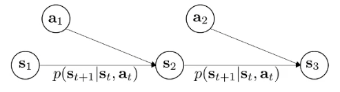
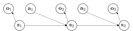
partially observed Markov decision peocess

$\mathcal{M}=\mathcal{S},\mathcal{A},\mathcal{O},\mathcal{T},\mathcal{E},r$
$\mathcal{E}$-emmision probobality $p(o_t|s_t)$

由于$a_t$是根据$s_t$和${\pi }_{\theta }$共同推出的：$p((s_{t+1},a_{t+1})|s_t,a_t)=p(s_{t+1}|s_t,a_t){\pi }_{\theta }(a_{t+1}|s_{t+1})$

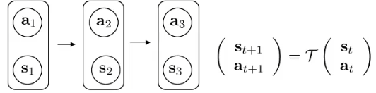
statinary: the same before and after transition: $\mu =\mathcal{T}\mu$，因此$\mu$是$\mathcal{T}$的特征值为1的特征向量！
for statinary distribution, $\mu =p_{\theta }(s,a)$
利用期望，是为了将不连续的奖励变成连续的变量，从而适用于梯度下降等算法

Value Functions

Q-function

$Q^{\pi }(s_t,a_t)={\sum }_{t^{\prime }=t}^T{E}_{{\pi }_{\theta }}[r(s_{t^{\prime }},a_{t^{\prime }})|s_t,a_t]$: 在$s_t$状态下执行动作$a_t$的所有奖励

value function

$V^{\pi }(s_t)={\sum }_{t^{\prime }=t}^T{E}_{{\pi }_{\theta }}[r(s_{t^{\prime }},a_{t^{\prime }})|s_t]$：$s_t$状态下的所有奖励（注意看自变量和它对什么去了取了期望）
So, $V^{\pi }(s_t)=E_{a_t\sim \pi (a_t|s_t)}[Q^{\pi }(s_t,a_t)]$，如果我们对状态再求一次期望呢？：
$E_{s_1\sim p(s_1)}[V^{\pi }(s_1)]$ is the RL objective (对所有可能的出发的状态进行求期望，就是我们上面说的goal)

Using $Q^{\pi }$ and $V^{\pi }$

• if we have policy $\pi$, and we know $Q^{\pi }(s,a)$, then we can improve $\pi$:
  • set ${\pi }^{\prime }(a|s)=1$ if $a=\arg {\max }_a{Q}^{\pi }(s,a)$
  • this policy is better than $\pi$
• compute gradient to increase probobality of good actions a:
  • if $Q^{\pi }(s,a)>V^{\pi }(s)$, then a is better than average 因为$V^{\pi }$是平均的各种动作奖励值
  • modify $\pi (a|s)$ to increase probobality of a if $Q^{\pi }(s,a)>V^{\pi }(s)$
    
    Q-value和V-value都是用来评价策略好坏的

Types of RL algorithms

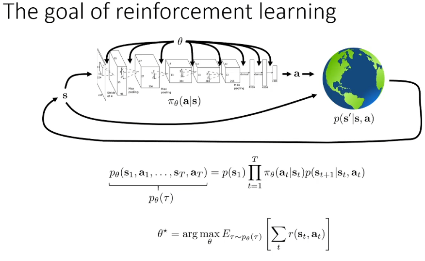
Our goal:
$${\theta }^{\ast }=\arg \underset{\theta }{\max }{E}_{\tau \sim p_{\theta }(\tau )}\left[\sum _{t}r(s_t,a_t)\right]$$

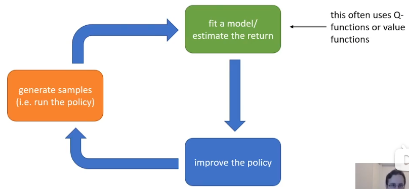
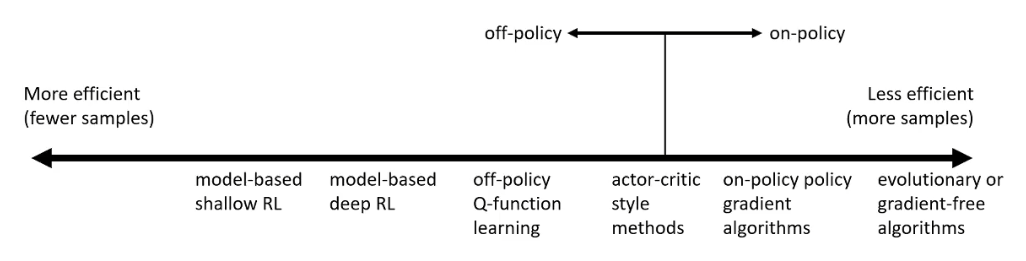
[!NOTE] Types of RL algorithms

• Policy gradients: 直接计算目标函数对$\theta$的导数，然后执行梯度下降
• Value-based: 为最优策略去模拟（神经网络去模拟）值函数或者Q函数。（没有明确的策略）
• Actor-critic: 上面两种的结合，模拟值/Q函数，然后去更新策略
• Model-based: estimate the transition model $\mathcal{T}$
  • 用它来planning（没有明确的策略）
  • 用来更新策略

Examples of algorithms

• Value function fitting
  • Q-learning, DQN
  • Temporal difference learning
  • Fitted value iteration
• Policy gradient methods
  • Reinforce
  • Natual policy gradient
  • Trust region policy optimization
• Actor-critic
  • A3C
  • SAC
  • DDPG
• Model-based RL
  • Dyna
  • Guided policy search

Policy gradient

我们对着这个幻灯片来讨论讨论：
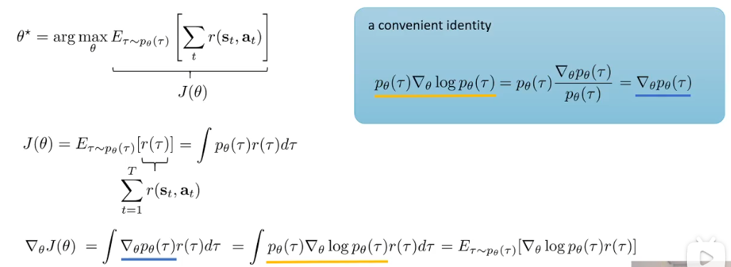
首先这个$J(\theta )$表示某个特定的策略的轨迹奖励，也就按照这个策略，跑完整个的所有reward
因为最终的目标就是找到最佳策略使得$J(\theta )$的期望最大，也就是说它就是优化函数，因此我们要对$J(\theta )$求导。
积分和求导符号可以换位置。要求期望就得知道概率分布$p_{\theta }(\tau )$，而这个是不知道的。因此利用了蓝框里的，对$p_{\theta }(\tau )$求导变成对$\log p_{\theta }(\tau )$求导，有了下面的：

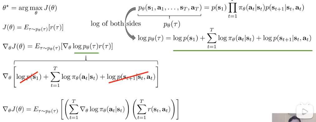
几个和策略$\theta$无关项求导之后都等于零，$p_{\theta }(\tau )$的展开又可以利用log转换为求和
因此得到最后一行，也就是剩下的参数我们都是知道的（$\pi$、$r$）

由于$J(\theta )$是个期望，那么就可以通过多次实验采样然后平均得到：
$${\nabla }_{\theta }J(\theta )\approx \frac{1}{N}\sum _{i=1}^N\left(\sum _{t=1}^T{\nabla }_{\theta }\log {\pi }_{\theta }(a_{i,t}|s_{i,t})\right)\left(\sum _{t=1}^{T}r(s_{i,t},a_{i,t})\right)$$

我们再对应着那三个box的颜色看看：

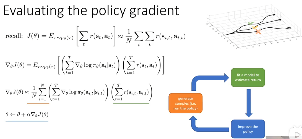
这里的${\pi }_{\theta }(a_t|s_t)$是什么？
可以是神经网络输出的概率（离散），
也可以是动作的概率分布（连续）：
${\pi }_{\theta }(a_t|s_t)=\mathcal{N}(f_{\text{neural network}(s_t)};\Sigma )$ （高斯分布例子）

把上面的式子稍微简化一点：
$$\begin{array}{rl}{\nabla }_{\theta }J(\theta )& \approx \frac{1}{N}\sum _{i=1}^N\left(\sum _{t=1}^T{\nabla }_{\theta }\log {\pi }_{\theta }(a_{i,t}|s_{i,t})\right)\left(\sum _{t=1}^{T}r(s_{i,t},a_{i,t})\right)\\ & =\frac{1}{N}\sum _{i=1}^N{\nabla }_{\theta }\log {\pi }_{\theta }({\tau }_i)r({\tau }_i)\end{array}$$

考虑到因果性：现在的决策不会影响过去的reward，绿色框中可以改写一下：
${\hat{Q}}^{\pi }(x_t,u_t)={\sum }_{t^{\prime }=t}^{T}r(x_{t^{\prime }},u_{t^{\prime }})$
我们把轨迹$\tau$写开，再利用因果性的$\hat{Q}$：
$${\nabla }_{\theta }J(\theta )\approx \frac{1}{N}\sum _{i=1}^N\sum _{t=1}^T{\nabla }_{\theta }\log {\pi }_{\theta }(a_{i,t}|s_{i,t}){\hat{Q}}_{i,t}^{\pi }$$
${\hat{Q}}_{i,t}^{\pi }$表示如果你在$s_{i,t}$状态采取$a_{i,t}$动作，并按照$\pi$策略继续下去跑完整个轨迹的奖励的估计。

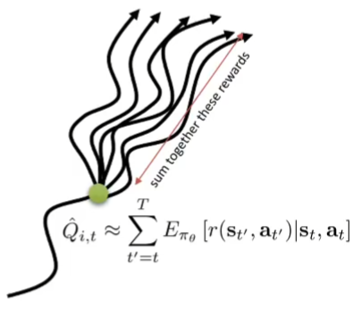
重点就在于求和的下标，这样做的最大好处就是能够减少有限样本带来的方差
其实policy gradient的原理就是在最大似然估计的基础上，按照${\hat{Q}}^{\pi }(x_t,u_t)$进行加权：

$$\tilde{J}(\theta )\approx \frac{1}{N}\sum _{i=1}^N\sum _{i=1}^N\log {\pi }_{\theta }(a_{i,t}|s_{i,t}){\hat{Q}}_{i,t}$$

大量有趣的数学技巧，包括为梯度和=增加约束

在L5，gradient policy的最后一节，Trust region policy optimization

Actor-critic

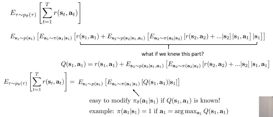
来个baseline，接着我们上面的说，正因为$\hat{Q}$只是多次采样的对期望的模拟，因此假设我们有一个理想的reward的期望:
$$Q(s_t,a_t)=\sum _{t^{\prime }=t}^T{E}_{{\pi }_{\theta }}[r(s_{t^{\prime }},a_{t^{\prime }})|s_t,a_t]$$
然后考虑在一个特定的状态$s_t$下，预期的所有动作的平均reward，就是值函数的定义（注意自变量和它是对谁取了期望）
$$V(s_t)=E_{a_t\sim {\pi }_{\theta }}(a_t|s_t)[Q(s_t,a_t)]$$
这个就可以作为我们的baseline，代表就是平均的行动回报：（代替原本的恒定的$b$）

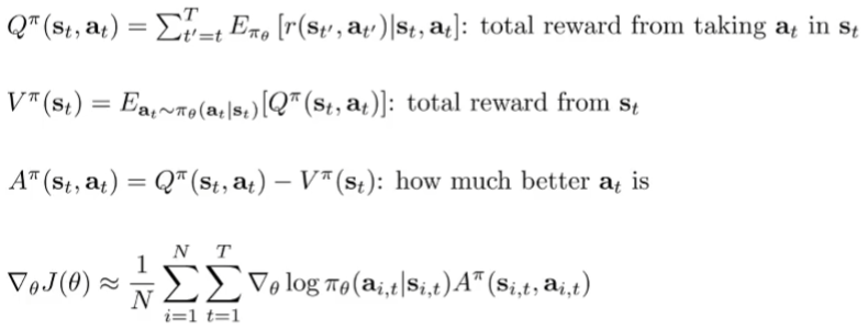
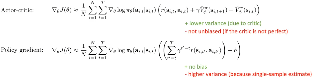
[!NOTE] AC和policy gradient的区别
所以以前的${\sum }_{t=1}^{T}r(s_{i,t},a_{i,t})$其实是一种蒙特卡洛估计，虽然无偏但是方差很大，我们用些许的偏差换来方差的巨大减小，也就是要直接去fit $Q^{\pi },V^{\pi },or{A}^{\pi }$. 因为后者本质是期望，哪怕是我们拟合的期望函数，也比采样得到的$r()$更好

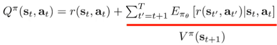
第一项实际上是确定的不是随机变量，因为是当下的状态和动作。$$Q^{\pi }(s_t,a_t)\approx r(s_t,a_t)+V^{\pi }(s_{t+1})$$ 这里进行了小的近似：从t到t+1的过程相当于用单样本进行了近似，因为理论上来说这里的状态转移也是要取期望的，随后就可以得到：
$$A^{\pi }(s_t,a_t)\approx r(s_t,a_t)+V^{\pi }(s_{t+1})-V^{\pi }(s_t)$$
$A^{\pi }(s_t,a_t)$意义是动作$a_t$比根据策略$\pi$产生的平均动作reward好多少：Advantage

A和Q都取决于两个变量：状态和动作，而V只取决于状态，因此更好去模拟fit——接下来就用基于V函数的critic

Estimate V

$V^{\pi }(s_t)\approx {\sum }_{t^{\prime }=t}^{T}r(s_{t^{\prime }},a_{t^{\prime }})$
not as good as: $V^{\pi }(s_t)\approx \frac{1}{N}{\sum }_{n=1}^N{\sum }_{t^{\prime }=t}^{T}r(s_{t^{\prime }},a_{t^{\prime }})$, but still pretty good
So, our training data: $\left\{(s_{i,t},{\sum }_{t^{\prime }=t}^{T}r(s_{i,t^{\prime }},a_{i,t^{\prime }}))\right\}$ ，右边的就是$y_{i,t}$
supervised learning: $\mathcal{L}(\varphi )=\frac{1}{2}{\sum }_i||{\hat{V}}_{\varphi }^{\pi }(s_i)-y_i|{|}^2$

algorithms-with discount

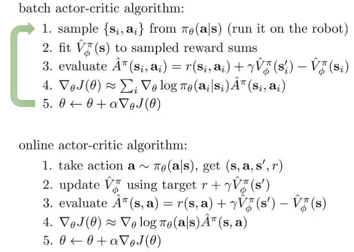
上面的方法需要我们去使用两个神经网络去拟合函数：
s->${\hat{V}}_{\varphi }^{\pi }$和s->${\pi }_{\theta }(a|s)$

原文地址：https://blog.csdn.net/QinZheng7575/article/details/140638246

免责声明：本站文章内容转载自网络资源，如本站内容侵犯了原著者的合法权益，可联系本站删除。更多内容请关注自学内容网（zxcms.com）！